A few posts back I was concerned with optimising the WiFi reception in my flat, and I chose a simple method for calculating the distribution of electromagnetic intensity. I casually mentioned that I really should be doing things more rigorously by solving the Helmholtz equation, but then didn’t. Well, spurred on by a shocking amount of spare time, I’ve given it a go here.
UPDATE: Android app now available, see this post for details.
The Helmholtz equation is used in the modelling of the propagation of electromagnetic waves. More precisely, if the time-dependence of an electromagnetic wave can be assumed to be of the form 


where 


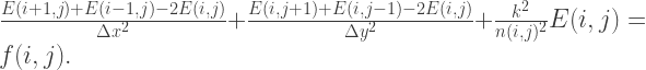
This is a linear equation in the ‘current’ cell 


This is slightly tricky due to the fact that a 2D labelling system 


A pair of cells 


The row in the matrix equation corresponding to the
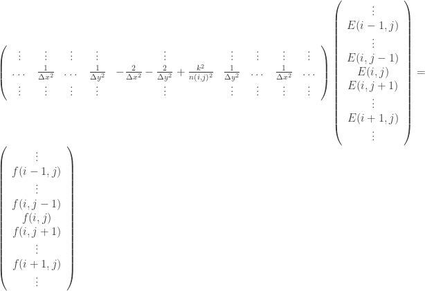
where there are 


Fortunately this problem has crept up on people cleverer than I, and they invented the concept of the sparse matrix, or a matrix filled mostly with zeros. We can visualise the structure of our matrix using the handy Matlab function spy – as plotted below it shows which elements of the matrix are nonzero.

Here 
Moving on to the physics then, what does a solution of the Helmholtz equation look like? On the unit square for large 
In this calculation I’ve set boundary conditions that 
Visualised below are a selected few pretty pictures where I’ve taken a logarithmic colour scale to highlight the positions of zero electric field – the ‘nodes’. As the animation proceeds

Once again physics has turned out unexpectedly pretty and distracted me away from my goal, and this post becomes a microcosm of the entire concept of the blog…
Moving onwards, I’ll recap the layout of the flat where I’m hoping to improve the signal reaching my computer from my WiFi router:

I can use this image to act as a refractive index map – walls are very high refractive index, and empty space has a refractive index of 1. I then set up the WiFi antenna as a small radiation source hidden away somewhat uselessly in the corner. Starting with a radiation wavelength of 10 cm, I end up with an electromagnetic intensity map which looks like this:

This is, well, surprisingly great to look at, but is very much unexpected. I would have expected to see some region of ‘brightness’ around the electromagnetic source, fading away into the distance perhaps with some funky diffraction effects going on. Instead we get a wispy structure with filaments of strong field strength snaking their way around. There are noticeable black spots too, recognisable to anyone who’s shifted position in a chair and having their phone conversation dropped.
What if we stuck the router in the kitchen?

This seems to help the reception in all of the flat except the bedrooms, though we would have to deal with lightning striking the cupboard under the stairs it seems.
What about smack bang in the middle of the flat?

Thats more like it! Tendrils of internet goodness can get everywhere, even into the bathroom where no one at all occasionally reads BBC News with numb legs. Unfortunately this is probably not a viable option.
Actually the distribution of field strength seems extremely sensitive to every parameter, be it the position of the router, the wavelength of the radiation, or the refractive index of the front door. This probably requires some averaging over parameters or grid convergence scan, but given it takes this laptop 10 minutes or so to conjure up each of the above images, that’s probably out of the question for now.
UPDATE
As suggested by a helpful commenter, I tried adding in an imaginary component of the refractive index for the walls, taken from here. This allows for some absorption in the concrete, and stops the perfect reflections forming a standing wave which almost perfectly cancels everything out. The results look like something I would actually expect:
END UPDATE
It’s quite surprising that the final results should be so sensitive, but given we’re performing a matrix inversion in the solution, the field strength at every position depends on the field strength at every other position. This might seem to be invoking some sort of non-local interaction of the electromagnetic field, but actually its just due to the way we’ve decided to solve the problem.
The Helmholtz equation implicitly assumes a solution independent of time, other than a sinusoidal oscillation. What we end up with is then a system at equilibrium, oscillating back and forth as a trapped standing wave. In effect the antenna has been switched on for an infinite amount of time and all possible reflections, refractions, transmissions etc. have been allowed to happen. There is certainly enough time for all parts of the flat to affect every other part of the flat then, and ‘non-locality’ isn’t an issue. In a practical sense, after a second the electromagnetic waves have had time to zip around the place billions of times and so equilibrium happens extremely quickly.
Now it’s all very well and good to chat about this so glibly, because we’re all physicists and 90% of the time we’re rationalising away difficult-to-do things as ‘obvious’ or ‘trivial’ to avoid doing any work. Unfortunately for me the point of this blog is to do lots of work in my spare time while avoiding doing anything actually useful, so lets see if we can’t have a go at the time-dependent problem. Once we start reintroducing 
This is exactly what the FDTD technique achieves – Finite Difference Time Domain. The FD means we’re solving equations on a grid, and the TD just makes it all a bit harder. To be specific there is a simple algorithm to march Maxwell’s equations forwards in time, namely
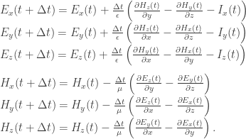
I’ve introduced a current source 


With the router in approximately the correct place, you can see the radiation initially stream out of the router. There are a few reflections at first, but once the flat has been filled with field it becomes static quite quickly, and settles into an oscillating standing wave. This looks very much like the ‘infinite time’ Helmholtz solution above, albeit at a longer wavelength, and justifies some of the hand-waving ‘intuition’ I tried to fool you with.

Great simulations 🙂 Thanks for sharing.
My only concern is the bandwidth of your signal . In most WLAN networks there is about 20MHz of radio bandwidth available. You may simulate this using different subcarriers at different frequencies, as in OFDM systems. Standard WLAN OFDM supports 52 subcarriers with 312.5KHz subacarrier spacing, i.e. from -26 to +26, avoiding zero, around the center frequency. Such a wideband simulation should have a big impact on the results.
Regards
LikeLike
Would it be appropriate to directly model the subcarriers as 52 narrowband sources in the E-field? I don’t know much, but reading the specs and documentation about OFDM in 802.11, the subcarriers are FFT’d to a 4us long frequency domain signal that is actually modulated onto the carrier. Looking a a spectrogram for a WiFi frame, it looks pretty uniform over fc+-9 MHz.
I’m trying to reproduce this myself (Helmholtz solution), but part of my problem is pinning down what to use as f(x) for the source, narrowband or otherwise. I’ve got a decent handle on the mathematics, but my EM physics is failing me…
One good thing: I doubt the refractive index of the materials involved is that intensely frequency dependent, so constant values (spatially varying) still seem ok.
LikeLike
Ooh, how are you introducing a finite bandwidth to the Helmholtz solution? For the FDTD method I added in some channels at +- 312.5 kHz as suggested, but over the length of the simulation (~ns) there wasn’t any difference – I guess there will be a modulation over timescales ~1/312.5kHz, but the simulation doesn’t get that far. If there’s a way of implementing it with the Helmholtz method then that’s the way to do it.
LikeLike
So here is what I’ve come up with. Its technically not the Helmholtz equation, but it is pretty close:
Assume a separable solution to the wave equation:
A(r,t) = A(r)A(t), as with Helmholtz.
Instead of assuming A(t) is of the form Re{e^(i*w*t)}, the new assumption is int( e^(i*w*t)dw,w-B,w+B), which is a perfectly reasonable linear combination of the general sinusoid shape. This is a uniformly distributed in the passband region around angular frequency w, with width 2B. Probably not perfectly realistic for the modulation scheme, but at least wideband.
Solving the wave equation with A(r,t) as above produces laplace(A(r)) = (1/(c^2*A(t) * d^2 A(t) / dt^2). Setting both sides equal to -k^2 (arbitrary choice, same as Helmholtz) yields the same spatial equation. However, the usual substitution of k=w*c doesn’t hold for A(t). Instead, we find that k^2 = ( w^2 + s^2/3)/c^2. I have yet to solve the spatial Helmholtz with the modified k, but this is the direction I’m leaning.
I’ve also toyed around with various other linear recombinations of sinusoids, including sum( e^(i*v*t), v = w-26*s, w+26*s) to model 52 different subcarriers centered around w. This yields k^2 = ( w^2 + 384 s^2) / c^2 .
My intuition of the Helmholtz solution isn’t very good, but this doesn’t seem like it will appreciably change the results. 20MHz out of 2400MHz isn’t much.
It is possible that there isn’t a separable solution as I assumed in the first step above… but my intuition is that eventually a standing wave will be established which is time independent.
I’m planning on using FEniCS as my PDE solver of choice; any experience with it?
LikeLike
Hmm… no way to edit comments, but I meant k^2 = ( w^2 + B^2/3 ) / c^2 for the uniform wideband frequency source.
LikeLike
You may dig into FDTD literature for implementation ideas. With 52 narrowband channels, the summation of the EM field strength from all subcarriers should give you an upper bound for the field strength at each point. In fact, the actual field is frequency dependent.
About OFDM spectrum, after IFFT there are additional filters, hence the spectrum is much smoother. However, what you see in the documentation is the spectrum mask. In practice there is a deep notch in the center and the power at each subcarrier is adjusted adaptively. However, any wideband model, as you suggested, should suit for this purpose.
And the outcome should be quite different between narrowband and wideband channels, depending on the environment. 20MHz is substantially wider than the coherence bandwidth of most urban radio channels. In an small flat model with non-reflective objects and weak transmit power the difference can be small. A realistic model, should incorporate some highly reflective metallic surfaces and the surrounding apartments as well.
LikeLike
I am genuinely grateful to the owner of this web
site who has shared this fantastic piece of writing at here.
LikeLike
I like readsing through a post that will make men and womjen think.
Also, many tnanks for permitting me to comment!
LikeLike
Thanks for this great post ! It is not often that math can be applied to resolve so neatly a very practical question.
Couldn’t resist making an ipython notebook out of it (in Julia) :
http://nbviewer.ipython.org/gist/fredo-dedup/31ae1b6017833e9a18f8
LikeLike
That’s fantastic! I’m glad you enjoyed the blog post. How large did you manage to make a room? Memory constraints were why I avoided using a sparse Helmholtz solver in the app.
LikeLike
I tried bigger rooms on a desktop with more RAM today :
At 1000×1000 pixels : allocated mem ~ 2Gb, 45 sec for solving.
And 2000×2000 pixels : allocated ~ 9Gb, 330 sec for solving
LikeLike
I tried to reply your results and I got this error:
”
In [23]:
f = fill (0. + 0.im (dim X, dimy))
f [80:82, 160: 162] = 1.0;
BoundsError ()
while loading In [13], in expression starting on line 2
in checkbounds at abstractarray.jl: 65
in setIndex! multidimensional.jl at: 61 ”
I posted that on https://groups.google.com/forum/#!topic/julia-dev/maBuEwR61NM, I will apreciate if you help me with that problem.
Sorry for my English.
LikeLike
Would it be possible to have multiple materials in your ipython notebook? it looks like a nice app, maybe it is worth to make it compatible with the floor plans used in WiFi Solver, the 5 materials used in WiFi Solver are enough.
LikeLike
I’m nnot that uch of a intrernet reader
to be honest but your sites really nice, keeep it up!
I’ll ggo ahead and bookmark your site to come back down the road.
Alll the best
LikeLike
Reblogged this on andronicas's Blog and commented:
Very interesting read
LikeLike
What effect do you think neglecting the third dimension has on the result?
Router and receiver might be at different heights, etc.
(Obviously computation time and memory are the main limitation)
Great post, enjoyed reading it.
LikeLike
There are quite strong reflections coming from the ceiling and floor. If the access point is very close to the ceiling or floor these reflections are very strong. In practice you always need a 3D model for realistic simulations. Moreover, the access point is not propagating uniformly in 3D. The antenna (combined with the device) has a pattern. If you keep the antenna vertical, propagation in horizontal plane is much stronger than the vertical plane, hence the walls play a bigger role than than the ceiling or floor.
LikeLike
At the end, what is more important is the material of the walls. If your ceiling has a metallic surface or metallic structure, but the walls are made of wood and plaster, then the effect of the ceiling would be much stronger. For a precise simulation you need to model every wall, window, door and furniture (e.g. fridge) with their specific parameters.
LikeLike
About the height, assuming dipole antennas at vertical direction, it is better to keep everything at the same height. The height of the device is very determining, especially with longer antennas that have a flat pattern. In close distnace line-of-sight scenarios, the effect of changing heigh could be much stronger than changing the location.
LikeLike
Reblogged this on The Cryptosphere and commented:
Math! Wifi! Optimization! Waaaaay more fun than it sounds! How to use math to calculate the best spot for your router, copiously illustrated and featuring the geekiest, prettiest gif you’ll see today!
LikeLike
Where is your android app? what is its name you made?
LikeLike
Here you go: https://play.google.com/store/apps/details?id=com.jasmcole.wifisolver
LikeLike
Please consider posting your Matlab code on the Mathworks file exchange. Other Matlab users like myself would enjoy playing with your code.
LikeLike
Unquestionably believe that which you said. Your
favorite justification seemed to be on the internet the
simplest thing to be aware of. I say to you, I definitely get annoyed while people consider worries that they just
do not know about. You managed to hit the nail upon the top and also defined out the
whole thing without having side effect , people can take
a signal. Will probably be back to get more. Thanks
LikeLike
Nice, looks cool.. Just a few questions, why is your source this big?? how did you model the antenna here, and is it made to resonate at 2.4ghz??
How is the space discretised? or how is the space(room) gridded? you talked about gridding down to millimeter but that you didn’t because of the computation time. Can you comment abouth how you set the time steps and space grids (dx and dy) versus wavelength??
LikeLike
Thanks. The source is actually 1 grid cell in size, approximating a delta-function source. In the Helmholtz case, I specify the vacuum wavelength when building the solution matrix, where it enters as ‘k’. In the FDTD case I directly update the source function (here a current density) every time step to oscillate at 2.4 GHz. In the post I use 20 grid points per wavelength (I think…), which is really a lower limit if you want semi-decent accuracy. The time step is then set to be slightly lower than the upper bound given by the CFL condition dt = 1/(c*sqrt(1/dx^2 + 1/dy^2)). If you’re attempting this you’ll notice with an FDTD solver the phase velocity is highest for waves at 45 degrees, so if you use too low a resolution the wavefronts will look square rather than circular. For the Helmholtz case the resolution was limited by available memory on my (suffering) laptop.
LikeLike
Can I simply say what a relief to discover a person that genuinely
understands what they are discussing online. You certainly realize how to bring an issue to light
and make it important. More people have to check this out and understand this
side of the story. I was surprised that you
aren’t more popular since you surely possess the gift.
LikeLike
How did you set up the shape of your room? To me this seems like the most interesting and difficult problem here.
LikeLike
Hi Dean, I just drew the room in 2D in Sketchup, then saved the outline as a .png. This has the added benefit of discretising the room onto a Cartesian grid automatically, which simplifies the setting up of the simulation. If you’d like to explore yourself, you can find a link to the Android app I wrote at the top of the post. Cheers.
LikeLike
Hi!
I think that for your flat a directional antenna (something like 90V /15H @-3dB) would be much more appropriate. Would be interresting to simulate that instead of an omnidirectional antenna. (BTW, If you would go to simulate that don’t forget to reduce the power to meet the regulations!)
LikeLike
Hi, that sounds like a good idea! I’m not an electrical engineer, so how would I go about constructing a directional antenna from current sources? Do I need some sort of phased array of oscillators?
LikeLike
Hello, your work inspired us to do our group project in our bachelor physics about this topic. I have a few question and was hoping you could help me:
1.) When using the seperable Ansatz the separation constant is k^2/n^2. But now n is a function of (x,y)? How can this be justified?
2.) How do you implement your Delta-Function/Peak? Do you just set one entry in f to be a very large Number or how do you do that?
3.) How much RAM do you have? Even though we use sparse matrizes too we already get ‘Out of memory’ error at 1m x 1m space with dx = 0.005 = 0.5 cm or something. We have 8GB Ram.
4.) We have the issue that our results vary by diffrent step-sizes. So for example h = 1/32 gives us a complete diffrent result than dx = 1/16 or 1/64. I think this has something to do with the implied boundary conditions that are E = 0 at the borders. (This is indirectly implied by using only the “delta function” as f on the right hand side). Boundary Value Problems tend to do silly things when being proposed not well-defined. Have you encountered similar problems and how did you ‘solve’ this? We tried using only k-values in such a way that the wavelength is fraction of the space (the idea came from the schrödinger equation for a free particle in a infinitly high pot).
It would be very much appreciated if you could comment or answer to those issues! Again: Awesome blog, thanks for the inspiration! This has really inspired me to dig into some numerical physics/mathematics!
Cheers, Korbinian and Fabian from Germany
PS: Also propably a rather stupid question: The ‘Wifi part’ goes into the equation by using k=2pi / lambda, right?
PS2: You said in ealier comments that you would someday upload your Matlab script. I would be especially be interested in your plot, because ours looks pretty poor with surf(X,Y,Z), colormap set to ‘hot’ and zscale is logarithmic.
LikeLike
Hi, glad you’ve been inspired to do some work on this, and that you enjoy the blog.
1) Thanks for asking this, you’ve made me realise there is a typo throughout the blog post – it should be n^2k^2, not k^2/n^2 in the Helmholtz equation. I believe I’ve used the correct version in my code, but typed it upside down elsewhere! I’ve typed out my derivation here from Maxwell’s equations: https://www.writelatex.com/read/rbxfyjcnjvkj, feel free to let me know if I’ve made any mistakes.
2) I set a single grid cell of f(x,y) to be nonzero. The exact value doesn’t really matter, you could also use a finite-size source too if you wish by filling in more values of f.
3) I have 8GB of RAM too, I can use an grid of 700×1200 and Matlab only reaches ~4 GB RAM usage, when you’re only using a 200×200 grid
4) I make this assumption because I have made sure the edges of my simulation area are covered by a thick region of absorbing material, which makes the E = 0 approximation a good one
PS) The WiFi part is to make this an interesting topic to everyone! It really corresponds to any oscillating scalar field, like waves on a membrane, earthquakes through the Earth etc. Here we know the frequency of WiFi, so yes we know which k_0 to use 🙂
PS2) Simple ‘imagesc’ or ‘pcolor’ command, using a colourmap called ‘fire’ from the program ‘ImageJ’.
Good luck with your project! I’ve seen this blog be set for homework as far away as Guatemala, and as nearby as Kings College London 😉
LikeLike
I wonder if it is worth solving maxwell equation in 3D with probabilistic methods (so solve it as particle equations) than using typical numerical methods as here.
Has anyone tried?
LikeLike
I’m not sure what you mean, but I am intrigued. I’ve heard of Monte Carlo integration techniques, is this like heat you’re talking about?
LikeLike
Yes. They are easy to implement and far more realistic conditions are possible to be set. It is of course a sort of brute force method (and can be implemented in parallel or distributed as well, so many computers can be used; for example, in this problem if we want really accurate solutions and we need a large amount of computing time we can crowd source it!). I found this which seems to solve a similar problem: http://onlinelibrary.wiley.com/enhanced/doi/10.1002/jnm.834
One of their old paper shows some pseudocode of this algorithm. http://www.sciencedirect.com/science/article/pii/S0377042705005480
By the way, great article and work. Thanks.
LikeLike
Not sure why this comment didn’t get in..any ways just in case,… for the 3D maxwell..
Yes. They are easy to implement and far more realistic conditions are possible to be set. It is of course a sort of brute force method (and can be implemented in parallel or distributed as well, so many computers can be used; for example, in this problem if we want really accurate solutions and we need a large amount of computing time we can crowd source it!). I found this which seems to solve a similar problem:http://onlinelibrary.wiley.com/enhanced/doi/10.1002/jnm.834
One of their old paper shows some pseudocode of this algorithm.http://www.sciencedirect.com/science/article/pii/S0377042705005480
By the way, great article and work. Thanks.
LikeLike
Awesome! I managed to get this going on Matlab too but the results aren’t so alike. I have two pretty straight forward questions if you feel like helping. I was wondering what your space discretisation is in and if your Wi-Fi source is just a delta function?
LikeLike
Hi There. It is a really awesome piece of work you had done here. Im trying to do a similar implementation using Matlab too. It would be interesting to add the effects of the type of radiator (for example, a dipole antenna, which the Electrical Field has an analytic solution).
LikeLike
Hi, thanks, and glad you like the work. The source here is really the 2D analogue of a dipole antenna. In 3D this antenna has a doughnut-shaped radiation pattern for a finitely-sized antenna. Here we’re effectively simulating an infinitely-long antenna, which radiates with cylindrical symmetry. If you want to see some other solutions of Maxwell’s equations calculated in a different way, see my post here on Synchrotron Radation (beware, large GIFs):
https://jasmcole.com/2014/12/13/synchrotron-radiation/
LikeLike
hello!
After reading your “Helmholtz equation derivation”, I have a question about that.
you have said ” If we assume that n varies slowly with respect to a wavelength, then we can drop this term.”
but the truth is that n varies very quickly between the wall and the air. How do you deal with it? And how do you set the refraction index map exactly?
thank you!
LikeLike
Good question, this is what we in physics would call “ignoring the difficult bits of a problem”. Upon writing out that derivation, I though it would be a good idea to do a follow up post where I compare the effects of the extra term, and whether it becomes negligible as the walls get ‘softer’. If you’re questioning my results (and you should!) I encourage you to try yourself. I set the refractive index map by simply drawing an image and loading it in as a 2D array. This is the same way the app works too.
LikeLike
but what should I do to take account of the second term? the real derivative of the refraction index is nearly infinity, right?
LikeLike
The refractive index is varying on a scale much shorter than the wavelength, so as long as computationally your grid cells are much smaller than a wavelength then approximating the discontinuity as sudden jump in refractive index from cell to cell should be ok. If you were worried you could do a convergence scan, either varying the scale length of the index jump, or varying the size of a grid cell.
I suppose mathematically you should integrate over a small surface enclosing the boundary to find the jump conditions, and apply those as boundary conditions. This is the kind of derivation for something like Snell’s Law, where we know the conservation equations for E and D either side of a boundary.
LikeLike
Thank you!
After trying it myself, I confronted with two new problems.
1. If I don’t want to take account of the second term, then I should make the refraction index varying slowly. I make the n^2 vary from 6 to 1 covering 50 cm. Do you think that varying slowly enough?
2. If I take account of the second term, then according to the formula you derived, I should also take account of the horizontal components as well as the vertical component, right? And that will make problems very very difficult.
LikeLike
Too bad the app crashes with larger floorplans… But, I was able to process two 1530×1530 graphic on a tablet and stitch a larger image together with pretty decent results though. Was able to grab the screenshots out of the root folder after I got them to show up and created a short video. Thought you might like to see people using it in action!
Now maybe… overlay a second wireless AP to cover the dark areas?
LikeLike
Hi, thanks for the comment, and sorry for taking so long to approve it. Unfortunately, Android apps are limited by the OS in the amount of RAM they can access – trying to allocate too much memory causes the app to crash (hence the in-app warning). One of these days, I’ll release a desktop version of the app which is more heavyweight…
Thanks for the video! I’m impressed with what you’ve managed to do with the app – how exactly did you split up the simulation domain into two pieces?
LikeLike
Hi there! Iam writing a report on this subject and i just wonder if i could use some of your pictures of the signals in my report? Ofc i will be leaving references for it and link it back to you. I would be very greatful if you could write me an email confirmation in this matter.
//Robin
LikeLike
Hi Robin, sure that’s fine, the images have been on enough other websites that I’m sure it doesn’t matter who else uses them :). Good luck with the report.
LikeLiked by 1 person
Hi Robin, I’d like to read it when it’s done, could you post the link here ?
LikeLike
Great post!
It would be neat to set the source intensity to a realistic value (I think it’s arbitrary in the simulation?) and use a relation between signal intensity and data-transfer rate to plot a heatmap of, e.g., Mb/s, or to make it more intuitive, figure out how big your homepage is and plot a heatmap of seconds per homepage-download 🙂
LikeLike
Thanks! It would be nice to benchmark this particularly simple model against measurements of data rate. As many microwave engineers have told me, signal intensity does not directly predict data rate (though it is correlated), but it would be nice to know just how good a predictor it is.
LikeLike
Great post!! has this solver been patented?
LikeLike
Thanks! It has not, the core algorithm has been known for decades – see the book by Allen Taflove, the ‘bible’ of FDTD solvers.
LikeLiked by 1 person
Thanks Jasmcole..! May I know the book name??
LikeLike
Replying here, as I can’t below. The book is ‘Computational Electrodynamics: The Finite-Difference Time-Domain Method’.
LikeLiked by 1 person
Thank you!!!
LikeLike
Gah. I have no idea what most of this math stuff means. But the visual is fascinating. Also, makes me a wee concerned about the physical impacts on my body sitting next to that router all day every day.
LikeLike