During one of my many spells stumbling around on the internet, I came across a very cool paper on modelling the trajectories of particles around black holes (bear with me…). It has all the required ingredients for this blog: maths, physics, nice pictures, and the chance to throw in a Muse reference. Let’s have a look.

Black holes, in case you aren’t aware, are the remnants of dead stars, stars so massive they have collapsed in upon themselves to an infinitely dense point. Their gravitational fields are too strong for Newton to keep up with, so we need to turn to General Relativity in order to examine their properties.

Einstein developed the Einstein Field Equations (the clue is in the name) which describe how the presence of mass distorts spacetime. More precisely the stress-energy tensor of an object, a mathematical structure encoding the mass and energy contained, defines the local structure of spacetime by modifying its metric. The metric in turn is another bit of maths which just tells you how to work out the length of lines. In the flat spacetime Newton was used to the metric is very simple, and in fact everybody knows it from the formula

where is the length of a line, and are the coordinate displacements – this is just Pythagorus’ theorem. In the limit that  this becomes a differential relation.  The metric defines a geodesic, which is the shortest path between any two points. In flat space this is just a straight line, on the Earth’s curved surface it is a ‘great circle’, which is the path that aeroplanes take to minimise fuel usage.

Around a black hole things become more complicated, but by calculating the geodesics it is possible to see which paths a particle will take. There is no real gravitational ‘force’ in general relativity then, you are simply free-falling all the time along the geodesics that matter and energy are imprinting on your local spacetime. The force you feel on your feet as you walk around is the resistance to your natural free-fall path to the centre of the Earth.

So, with that out of the way, the authors of the paper I mentioned are concerned with the paths particles take around a cluster of black holes. It turns out that there is a surprisingly simple metric for this, the Majumdar-Papapetrou metric

where

and we have black holes at positions with masses . This metric is static, which means the black holes don’t move around. This is a good approximation if the particle moves over a timescale shorter than the black hole orbital timescale.

Letting the authors do the hard work for me, the equations of motion for a neutral particle in 2D with position and momenta  are

.

As everything in relativity is, well, relative, these momenta are the ones which would be observed by someone at rest with respect to the metric. The derivatives are taken with respect to the proper time of the particle. The actual velocity is . Knowing the equations of motion, I can set up some black holes, stick in a particle and see what happens using whichever ODE integrator methods tickle our fancy. Let’s start the particle at rest between the two black holes and see where it goes. The starting position I’ll call . Red stars mark the black hole positions, and the triangle is the starting position of the particle.

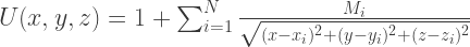
Naturally, due to the symmetry involved, it flies straight through and out the other side. If we move it up a bit:

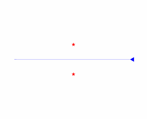
Again, unsurprisingly, it is captured by the black hole nearest to it. Keeping it still in the top half of the plane, there are also trajectories like this one where the particle swoops round into the other black hole.

In fact, it can be difficult to predict which black hole the particle will end up in, if its initial position changes even by a small amount, it can switch between the two – see the animation below . This is exactly the hallmark of a chaotic system as the authors of the paper point out.

In fact we came across this type of behaviour before on this blog, when I was talking about Newton fractals. There we picked some initial conditions and iterated a complex mapping, and our point moved around until it settled at a particular place. An equivalent thing is happening here, but instead of a complex map there is a system of differential equations. The concept of a basin of attraction is therefore useful again here – regions of phase space which send a particle to one black hole or another. In the Newton fractal it turns out that the basins of attraction have fractal boundaries for most polynomials. The same is true here, I’ve plotted below a small region of phase space where black means the particle ended up at one black hole, and white the other.

This shape has some strange properties, however far you ‘zoom in’ you can always find some holes or gaps. For this reason it isn’t quite two dimensional, but then again neither is it one dimensional as it can have some thickness. Rather, it has fractal dimension 1.43 as calculated in the paper, something in between a line and a plane. In fact, if you haven’t already you really should have a flick through, the authors manage to find some beautiful structures. In a very real sense though this object is one defined purely mathematically and deterministically, you really have to go in and explore it to see what surprises are in store. I encourage all of you with the means to simulate this to have a go – my code is attached at the bottom of the post.

I’ve also plotted below a selection of actual paths from this calculation. At this scale it looks like they all come from the same point, but actually they’re displaced very slightly. A very small displacement then leads to a wildly different path, chaos again! In fact the authors predict just how sensitive this system is to displacements in initial conditions, in terms of something called the Lyapunov exponent. This measures how quickly two similar trajectories diverge, and you may be interested to know for this system it is , something the authors verified numerically.

That takes a long time to compute though, for every point one must integrate a set of differential equations for many time steps. Instead let’s have a look at some nice trajectories:

And some with lots of black holes:

If you’d like to try this for yourself in Matlab, try the code here, unfortunately attached as a Word document as that’s all I’m allowed. You’ll need to supply

• xbh – vector of black hole x positions. I used (0,0)
• ybh – vector of black hole y positions. I used (-1 1)
• M – vector of black hole masses. I used (1/3,1/3).
• x0 – initial x position of particle
• y0 – iniial y position of particle
• ux0 – initial x velocity of particle
• uy0 – initial y velocity of particle
• plotflag – whether to plot or not, 1 or 0

Let me know if you get any nice trajectories!