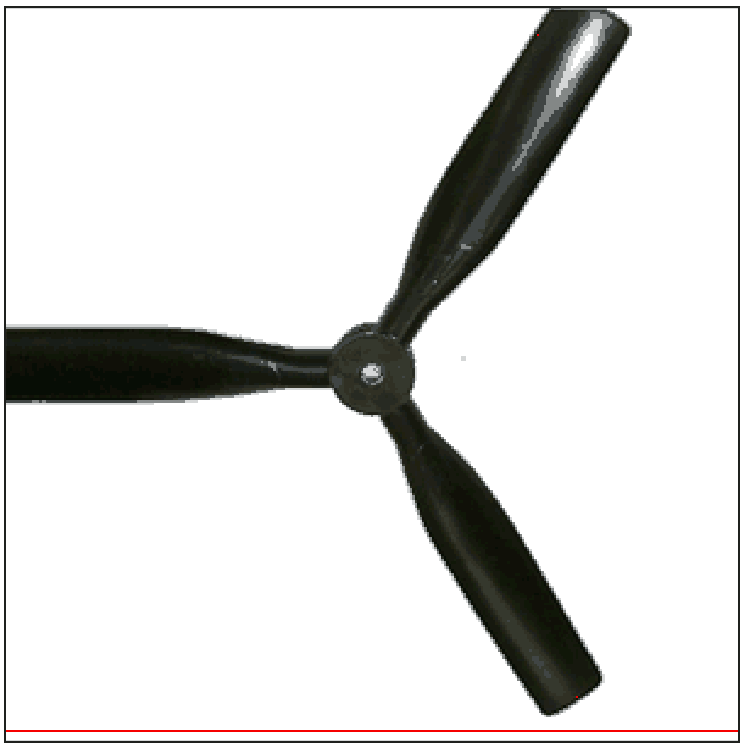
I remember seeing once the following photo from Flickr, and having my brain melt slightly from trying to figure out what went wrong:

The issue was the propeller was rotating as the camera detector ‘read out’, i.e. there was some motion during the exposure of the camera. This is an interesting thing to think about, lets have a look.
Many modern digital cameras use as their ‘sensing’ device a CMOS detector, also known as an active-pixel sensor, which works by accumulating electronic charge as light falls upon it. After a given amount of time, the exposure time, the charge is shifted row-by-row back to the camera for further processing. There is then a finite time where the camera scans down the image, saving rows of pixels at a time. If there is any motion over this timescale the image will be distorted.
To illustrate, consider photographing a spinning propeller. In the animations below the red line corresponds to the current readout position, and the propeller continues to spin as the readout proceeds. The portion below the red line is saved as the captured image.
First, a propeller which completes 1/10th of a rotation during the exposure:
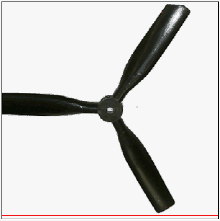
Some distortion, but nothing crazy. Now a propeller moving 10 times quicker, which completes a full rotation during the exposure:
This is starting to look like the Flickr image at the beginning. 5 times per exposure:
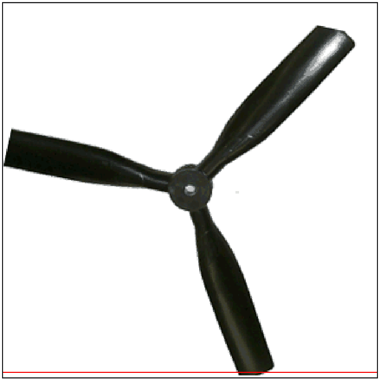
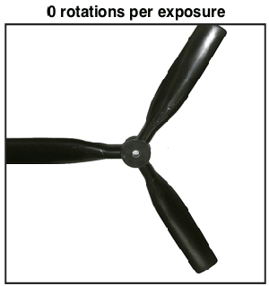
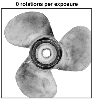
This is a little too far, things have clearly gone mental. Just for fun, let’s see what some different objects look like at different rotation speeds, from 0 to 1 rotation per exposure.
The same propeller as above:
A fatter propeller:
A car tire:

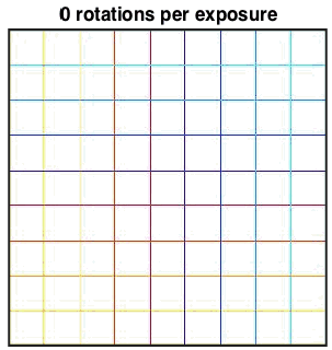
We can think of the rolling shutter effect being some coordinate transformation from the ‘object space’ of the real-world object, to the ‘image space’ of the warped image. The animation below shows what happens to the Cartesian coordinate grid as the number of rotations is increased. For small rotations the deformation is slight, as the number increases to 1 each side of the grid is moved successively towards the right-hand side of the image. This is a fairly complicated transformation to look at, but simple to understand.
Let the image be denoted by 


The object is rotating at angular frequency 


which is the required transformation. The factor 
To get some insight into the apparent shapes of the propellers, we can consider an object consisting of 


or
In Cartesian coordinates this becomes
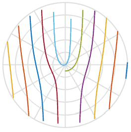
which helps to explain why the propellers get that S-shaped look – it’s just an inverse tangent function in the image space. Cool. I’ve plotted this function below for a set of 5 propeller blades at slightly different initial offsets, as might be observed during a video recording. They look pretty much like the shapes in the animations above.
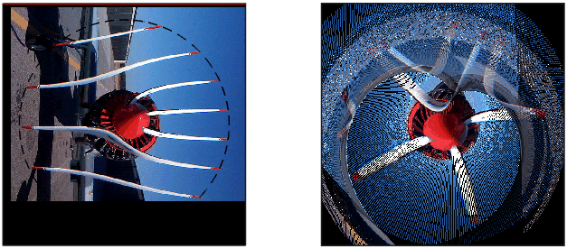
Now we understand a little more about the process, can we do anything about these ruined photos? Taking one of the warped images above, I can take a line through it, rotate backwards the appropriate amount, then stick those pixels onto a new image. In the animation below I scan through the image on the left, marked by the red line, then rotate the pixels along that line onto a new image. This way we can build a picture of what the real object looks like even if a pesky rolling shutter ruined our original image.
 Now if only my photoshop skills were better I could extract the propellers from the original Flickr image, un-warp them, and slap them back on the photo. Sounds like a plan for the future.
UPDATE:
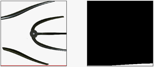
Some kind commenters were good enough to extract the propeller blades for me. To figure out the real number of blades and the rotation velocity we can look to this excellent post at Daniel Walsh’s Tumblr blog here, where he definitely has the edge on mathematical explanation. He works out that we can calculate the number of blades by subtracting the ‘lower’ blades from the ‘upper’ blades, so in this picture we know there should be 3. We also know the propeller is rotating approximately 2 times during the exposure, so if we try ‘undoing’ the rotation with a few different speeds around that we get something like this:
I’ve had to guess where the centre of the propeller is, and I’ve drawn a circle to guide the eye. Looking at that, the centre shouldn’t be too far off. There is unfortunately a missing blade, but there’s still enough information to make an image.
There is a sweet spot where everything overlaps the most, so picking this rotation speed (2.39 rotations per exposure), the original image and blades look like this:

It’s still a bit of a mess unfortunately, but at least looks something like the real object. Thanks commenters, and the comment on Hacker News where I saw the link to Daniel’s post.

Here’s the propeller, extracted. https://i.imgur.com/032Xksu.png
LikeLike
Thanks! I’ll have a look and update the post.
LikeLike
here are the props to your plane http://imgur.com/3tuKlJr
LikeLike
Thanks!
LikeLike
Props to you for doing that!
LikeLike
I gave up thinking of a pun for a post title this time, thanks for righting that terrible wrong.
LikeLike
…or writing a terrible wrong. 😉
LikeLike
that was great! what would that image look like when passed by the reversed filter? not just the propellers, the whole of it 😀
LikeLike
Hi,
Instead of extracting the propellers from the original image, maybe you could first blindly apply your last transformation to the first image, without any extraction first. Yeah, of course, it will probably do some funny transformation to the plane itself and the background, but 1/ you should get the original propellers in the middle of the reconstituted image, 2/ it would make another funny picture, and 3/ I’m curious about the result :-).
LikeLike
I wrote an education paper about an exercise you can do with this effect and a guitar:
http://iopscience.iop.org/0031-9120/49/4/431/article?fromSearchPage=true
If you turn the exposure time on a standard CMOS (the one in a mobile phone will usually allow you to) right down and look at guitar strings as they are played you get some very funky effects.
LikeLike
Nice! Is it my imagination, or are the low-frequency strings not making a perfect sinusoid? Is this because the (long wavelength) wave is travelling? If so, can you measure the wave velocity by working out how it would distort a sinusoid?
LikeLike
I wonder what happens with, say, a violin string.
LikeLike
What would it look like with a leaf shutter and with a focal plane shutter?
LikeLike
I work in visual effects and rolling shutter, mostly undesirable, is part of some renderers!
https://support.solidangle.com/display/AFMUG/Cameras#Cameras-RollingShutter
LikeLike
There’s a use for everything!
LikeLike
Reblogged this on A walking and Talking Duck and commented:
This is really pretty neat. I had no idea a CCD readout could distort rotational motion!
LikeLike
nice
LikeLike
Hi, I would like to ask about the mathematics. I don’t fully understand the transformation I(r,θ) –> f(R,Θ). How the images created was by stopping/freeze the coordinate I(r,θ), when the line pass through the corresponding coordinate. From your explanation (equation), looks like there is no requirements for this. Can you explain a little bit more? and how did you simulate the image of blade moving with different color?
LikeLike
Hi, the animations might be confusing you slightly. In the animation I effectively evaluate the co-ordinate transformation 1 line at a time. You can think of ‘f’ representing the image at the beginning of the animation. For every line, ‘f’ is rotated slightly and then ‘I’ (the final image) takes those values of the rotated ‘f’ along a line of constant y. The co-ordinate transformation is just another way of writing this, it doesn’t need to progress ‘line by line’, for every pixel in ‘I’ it tells us which colour it should be based on the pixels in ‘f’.
For the analytic solution of a propeller, I took ‘f’ to be nonzero only along lines of theta = constant for a few selected angles. Offsetting these angles slightly forms the animation.If you were to substitute theta = constant into the co-ordinate transformation, and switch to Cartesian co-ordinates, you’ll recover the equation for a propeller blade in ‘I’.
LikeLike
Reblogged this on Para Ser Piloto and commented:
Um efeito que eu nunca entendi por que acontecia – e acho que vocês também não… Agora finalmente desvendado!
LikeLike
For most digital cameras, select the lowest ISO speed on the camera, probably 50 or 100, then hold a +4 ND neutral density filter in front of the lens, and that should result in a slow enough effective shutter speed to get a normal prop blur. And let’s be honest here, “phones” really don’t make great cameras….
LikeLike
Michael Golembewski uses this principle and a flatbedscanner to create art:
http://golembewski.awardspace.com
LikeLike
Thanks for the interesting link
LikeLike
This is an absolutely brilliant article. The examples you create to illustrate your point are truly stunning. Thank you!
LikeLike
Thanks! Glad you like the post.
LikeLike
I don’t understand the coordinate transform. Could you explain it better for me? Why was only the angle affected? How do you describe this kind of coordinate transform using matrices? I would be very glad if you could explain it more to me. i wanted to use this concept of 2d non linear transforms for my maths exploration, but I don’t really understand it. Thanks
LikeLike
Hi, because we are modelling something spinning around the r = 0 point of the image, in the rolling shutter effect the r-component of the image isn’t affected, only the theta-component. The rolling shutter simply defines at which angle the image is ‘saved’, and this angle changes as a function of the position in the image. As the speed of the rolling shutter v increases, the coordinate transformation reduces to the identity and the effect is diminished. The transformation can’t be represented as a matrix because it is nonlinear in the image coordinates.
LikeLike
Now I wonder what these images would look like if scan lines were read in steps, e.g. always adding a number to the line number and doing modulo the sensor size, picking numbers that will read all the scan lines.
LikeLike
Hi, how did you create the animations of the spinning propeller at the top? I was wondering if I could do something similar in GeoGebra but I’m not sure how to plot the polar functions of the spinning propeller.
LikeLike
Hi, I used Matlab to make all of the animations here. For that one, in every frame I rotated a bitmap image slightly and ‘froze’ a line of pixels at a time, adding a red line to indicate the progression of the rolling shutter. From what I can see GeoGebra looks like it just plots curves? Matlab is expensive, but you can also look at Octave or Python which are free and just as easy to use.
LikeLiked by 1 person
hello, I’m working on it with Matlab recently as interests. But I cannot figure out this rolling shuttle artefacts phenomenon in Matlab. Could you share your code if possible?
LikeLike
Hi, thanks for your interest in this article. I hope to gradually add scripts from these blog posts to my github repository here
I haven’t put much there yet, but keep an eye on it for when I get round to cleaning up all my scripts and uploading them.
LikeLike
Here is an interactive GLSL shader I found demonstrating the concept: http://glslsandbox.com/e#29719.1
LikeLiked by 1 person
That’s fun to play with, thanks!
LikeLike
Inspired by your article, I built an interactive Version of a rolling shutter visualization in a Tool called GeoGebra recently by using line intersections. You can take a look at it here:
https://tube.geogebra.org/m/2294477
And the 3D Software Blender (really good stuff!) supports rolling shutter for 3D rendering since the last Version (2.77) as well. More details here: http://adaptivesamples.com/2015/12/08/rolling-shutter-coming-to-cycles/
Nice article and materials!
Regards,
Michael
LikeLike
Hi Michael, thanks for the link, that’s really nice interactive version. Are the ‘warped’ propellers pre-computed, or generated through line intersections? I have seen the rolling shutter effect in Blender, you might have noticed from my other posts that I am fond of playing around with it 🙂
LikeLike
This is very interesting, thank you for posting! I was hoping you could explain a point of the transformation for me…
Why is the distance that the shutter has traveled at (r, theta) y=rsin(theta)? Is this assuming that the shutter starts as the line y=0? What if the shutter where to start at y=-1? Would the distance traveled at position (r, theta) then be y=rsin(theta)+1?
Thank you in advance! Great stuff!
LikeLike
Hi Chris, good question and I’m glad you like the post. You are correct that the relation would be different for different choices of t = 0. Here I have taken t = 0 to correspond to the point where the shutter is halfway up the image. If, say, I were to pick t = t0 at this point, then the ‘time elapsed’ would be r*sin(theta)/v + t0, and the ‘number of radians’ would be omega*(r*sin(theta)/v + t0). This is different by a constant factor of omega*t0, and so the image transformation picks up and extra constant rotation factor. Finally, this just corresponds to choosing a different initial rotation angle for the image. The ‘rolling shutter’ version of the image will look similar, but the rotation advanced some amount of extra phase. There is no material difference, hence I chose t0 = 0 to avoid confusion. Hope this helps clear things up!
Jason
LikeLike