As the old saying goes, you wait ages for a bus and then two come along at once (or more!). Is this true though? My own anecdotal evidence would suggest yes, every single bloody time. However, we love data and maths in this blog almost as much as we hate waiting for the bus, so let’s have a more thorough look at the issue.

My data source in this post comes from Transport for London’s excellent developer feeds, where if you sign up, you can access live updates of the positions of every bus in the city. How cool is that? I thoroughly encourage you to go and have a poke around, if that’s something which takes your fancy. I’m using here Python (sorry Matlab), and the Matplotlib and Seaborn plotting modules, along with Numpy for the occasional bit of numerics.

First things first, what does the London bus network look like? Below I’ve roughly plotted all 512 routes, all overlaid on one another in different colours:

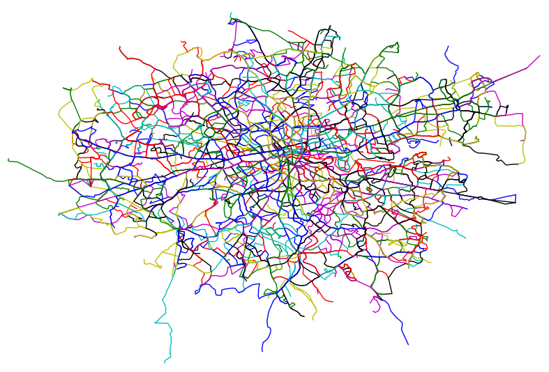Surprisingly, the bus network is so dense that it’s actually fairly difficult to make out the layout of the city. My main guiding features are the blank space corresponding to Richmond Park in the south west, and the characteristic (and bridgeless) loop of the Thames around the Isle of Dogs to the east. There are a few errors in the plot (the long straight sections), but it’s really just meant to give you the impression of how dense a good public transportation network needs to be in a big city.

I now change tack, and rather than approaching the data at the route level I move to the individual stop level. TfL provide a feed for the arrival time of every bus in the network at every relevant stop for up to 30 minutes in the future. This equates to a list of 88,000 or so bus stop arrival times, which I plot in two different ways below:

If we just look at every single arrival time at every single stop, we can bin those arrival times into bins spaced by 5 second increments and plot the resulting histogram as the blue curve above. This is multiply-counting buses, as they may appear as arrival times on several stops, but it should serve the impression that there is a near-constant stream of buses arriving at bus stops on average.

This, however, isn’t what the impatient commuter wants to know. Presumably they are waiting for a single type of bus, and would like to know for a particular stop how long until the next one (there may be multiple buses a commuter will want, but we’ll ignore that possibility for now). The green histogram therefore only includes, for each stop and each route servicing that stop, arrival times for the next bus of that route. This has a distribution which is much more like what we’d expect – odds are the buses will arrive sooner rather than later. In fact, the distribution looks convincingly exponential which we’ll come to later.

For now, lets look at the cumulative distribution function of the waiting times until the next bus:

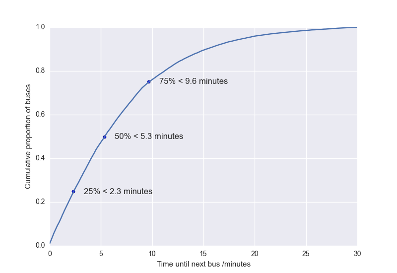I’ve labelled a few useful points – 50% of buses arrive within ~5 minutes, 1 in 4 arrive within ~2 minutes, and 3 in 4 arrive within ~ 10 minutes. By the time you’ve been waiting 20 minutes, your bus is now in the bottom 5th percentile of punctuality, and worse is probably packed and smelling of fried chicken.

These are all pretty solid stats for TfL (especially compared to other cities in the UK), but they’re really not what we care about at all. We would like to know why so many buses arrive in twos, or threes, after waiting ages for a single one. I mean, what are the odds?

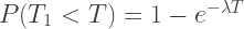
This is another question we can answer with our lovely data, and is plotted attractively (though with questionable utility) as a bivariate kernel density estimation below. Darker colours correspond to a high proportion of buses in that region of parameter space.

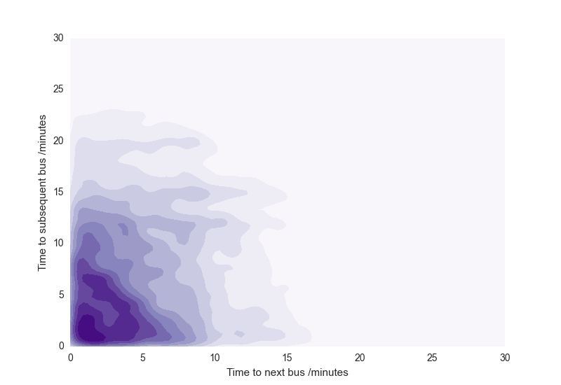As we saw above, most buses are concentrated near a short waiting period and drop off exponentially. There are some obvious peaks for differences in bus arrival times of 8, 12, 15 and 20 minutes, the standard intervals between the buses on most routes. Scandalously however, there are a significant number of buses for which the next one will arrive in > 10 minutes, and the subsequent one will arrive in less than 1 minute! Also, a lot of buses are arriving in a configuration where the first is arriving in less than 5 minutes, but so is the subsequent. Shouldn’t the bottom left of the plot be a bit more ‘thinned out’ if the buses are meant to be evenly distributed?

Here we need to turn to a bit of statistics, as our brains aren’t great when it comes to intuiting things like probabilities. The clue should come from the exponential shape of the ‘waiting’ distribution of the bus arrival times above. Though buses are ‘injected’ into the road network at uniform intervals, they are perturbed by traffic and bus stops and so can be thought to ‘thermalise’ into a less uniform distribution.

In the limit that the bus arrival times are random (an eminently sensible suggestion any commuter would agree with), we can approximate their arrival at a particular bus stop as a Poisson process. That is to say, the probability of buses arriving during a time period is given by

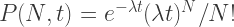
where is the average rate of arrival of the buses. Average in this sense means that in time , the average number of buses to arrive is

Crucially however, there is a nonzero chance of buses taking much less time to arrive, and also much more. What are the odds of no buses arriving in time ? This is

This is also the same probability that the first bus arrives at some time later than . Let the time of the first bus arrival be . Then

so

but we recognise that this is just the cumulative distribution of , so we differentiate to get the probability distribution of the arrival time of the first bus:

Great! This is the distribution we observe in the real London bus network, and indicates the underlying bus arrival process is Poisson (and therefore is about as random as nuclear decay). From the exponential fit we get buses/minute, or one bus every 7.5 minutes on average. This is about what I’d expect given the standard London bus timetables.

We shouldn’t get too happy though, as an exponential distribution exhibits a property known as ‘memorylessness’. That is, each bus arrival is an independent event and doesn’t affect the next bus arrival. To be concrete, suppose we’ve been waiting at a bus stop for a time , and no bus has arrived yet. Does this mean it should arrive sooner? The probability that it will arrive in a subsequent time interval is given by

which is exactly the same as if we’d only just arrived at the stop! This lack of memory means that at a given time, a Poisson process doesn’t depend in any way on the history of events, but just the time interval from now.

Is this really true for real buses, with their schedules and finite number? From the above we know that the joint probability of a bus arriving after a time and a second after a subsequent time is just given by

We’re interested in the likelihood of , the ‘two buses arriving at once’ case. Looking at an annotated version of our earlier plot, we see there are quite a few buses in this population:

Let’s get specific and choose some ratio , and we want to know the likelihood that the subsequent bus shows up times as quickly as the first one. If and the first bus shows up in 10 minutes, that means the second only takes 1 minute to arrive after that. We therefore need to integrate over the plane in the dashed triangle indicated above, so our probability is given by the double integral

which comes out to

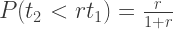
a nice simple result. The odds that the next bus makes us wait at least as long as the first is 50% as we might imagine. The odds that the next bus will arrive in a time less than one tenth of the first is around 9%, which is quite a lot! One in ten bus journeys may conceivably be plagued by the ‘two at once’ curse then, by our model anyway.

Let’s compare this to the TfL data:

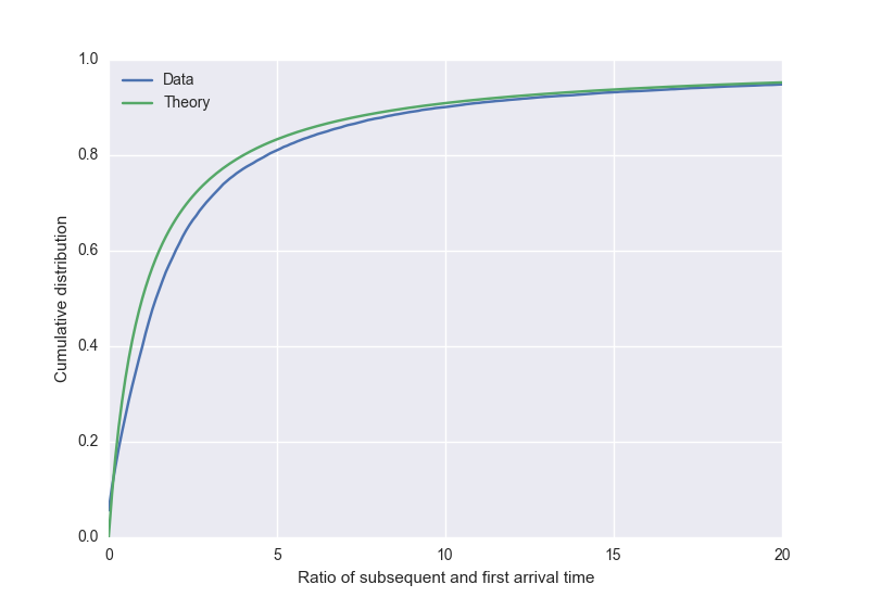
That’s not a bad match! Unfortunately for us, we’ve now compounded our evidence that the bus network, at least in a dense highly-perturbative road network such as London’s, is effectively random.

+1 for statistics, -1 for getting to work on time.