This blog has been getting a bit too pop-science for my tastes recently. Card games? Word clouds? Urgh. Let’s do some proper physics. I hope you’re paying attention at the back.

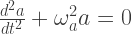
I’d like to talk about dispersion relations. As an illustrative example take the humble simple harmonic oscillator, where the position of something () is governed by the ODE

where is the natural frequency of the oscillator. If left by itself, this ODE states that will simply oscillate harmonically (hence the name) at frequency . If we want to know the behaviour of at different frequencies, we could apply them all at once and observe the resulting motion, which means solving

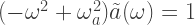
The -function represents the action of an infinitesimally short impulse to at . The simplest approach is in Fourier space, so after a Fourier transform the ODE becomes

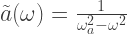
where and the Fourier transform of a delta function is constant in frequency space. Solving for the amplitude of ,

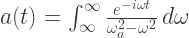
and inverse Fourier-transforming back to obtain the temporal motion,

The subsequent motion is therefore composed of a sum of oscillations at different frequencies , but the amplitude of each is weighted by how close is to the natural frequency. The farther from , the lower the amplitude of the oscillation. This is a more precise statement of the fact that the oscillator ‘wants’ to move at its natural frequency.

This statement can be generalised. Consider a system governed by some linear differential operator

We again take the Fourier transform of both sides, rearrange, and transform back:

Here is the dispersion relation corresponding to the operator , and in general the motion of is dominated by frequencies which cause to be as small as possible. In the SHM case implies .

Let’s add a little complexity to the simple case. Consider two oscillators and which are coupled together, i.e. the motion of one drives the motion of the other. The strength of this coupling is given by the constants and :

Now with two degrees of freedom the motion is represented by a vector, and the linear operator by a matrix:

For the motion not to be trivial, the determinant of the matrix should be zero, which leads to the coupled dispersion relation

where the frequencies of the two oscillators are and . If the couplings go to zero, then factorises to the two independent dispersion relations for the two oscillators, .

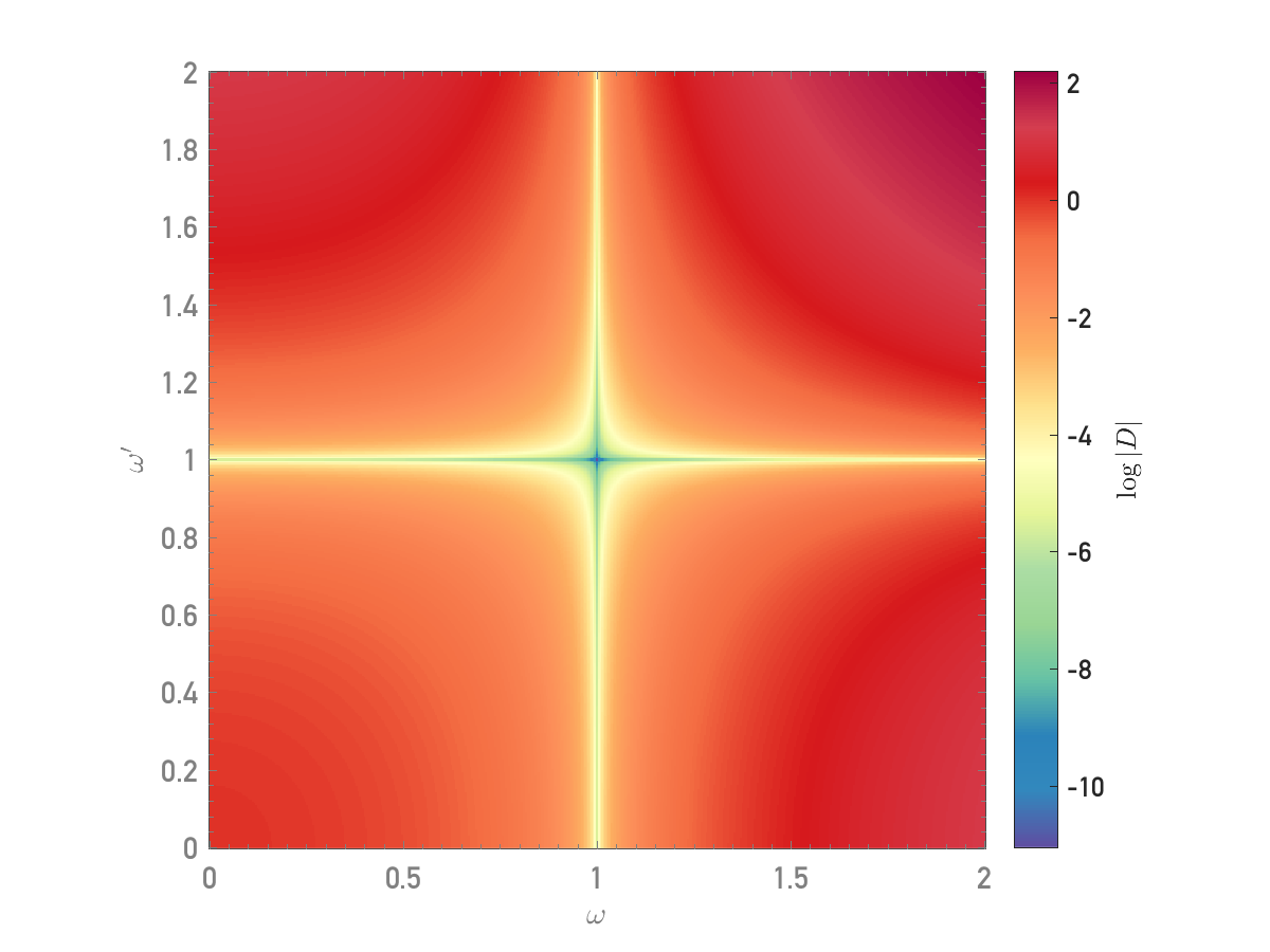
Let’s see what looks like in this case:

 

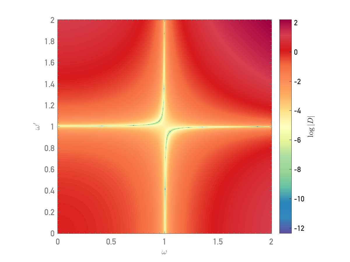
Everything looks normal. is minimised when both oscillators move at their own resonant frequencies. Let’s add some coupling:

This is interesting. At the resonant frequencies of the oscillators, it’s no longer possible for to be small. The problem is that we’re missing a chunk of the space that lives in. Let’s allow one of the frequencies to be imaginary, e.g. set .

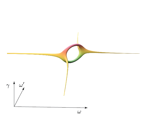
The dispersion relation is now 3-dimensional, so we can’t visualise it in the same way. Here I’ve picked the isosurface of evaluated at , and rendered it below using Blender:

Now we can see what has happened – our coupled system was forced out of the real plane near resonance, and the dispersion relation has had to develop branches above and below the real plane. Farther from resonance the branches fall back to the real plane, where they merge back into the real dispersion relation.

Let’s see what happens as we increase and decrease the coupling strengths:

Stronger coupling pushes farther out of the real plane, forcing the frequency of the oscillator to have larger imaginary component.

This is all very pretty, but let’s not forget the purpose of this post: hardcore physics. Back to the maths, let’s suppose that isn’t too large, and so the two oscillators are near their resonant frequencies.

Explicitly let have frequency and let have frequency . Substituting into the dispersion relation,

Assuming , then after multiplying out and discarding the higher-order terms,

This is a very useful expression. If the couplings are the same sign, then is imaginary and the effect of the coupling is to alter the frequencies of the oscillators. If the couplings are opposite signs then is real, and so represents an exponentially growing solution.

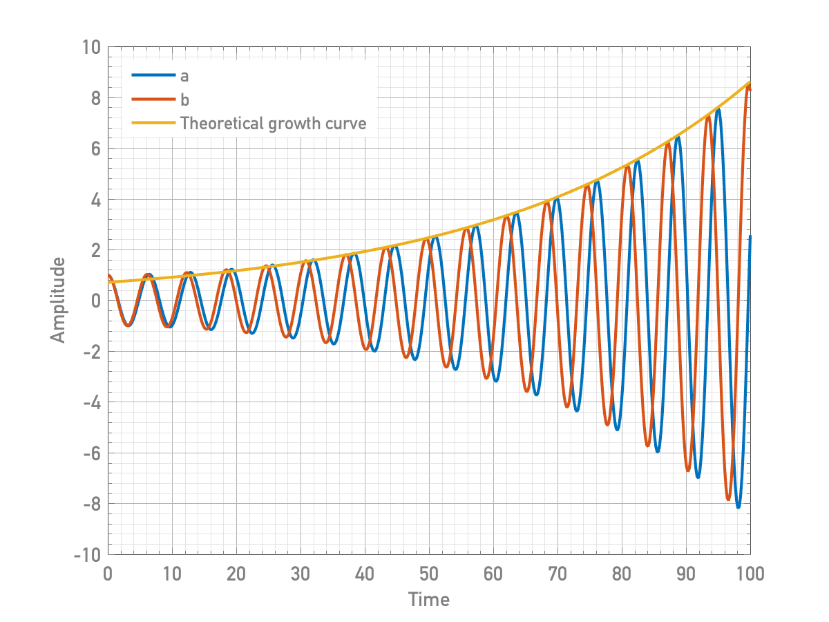
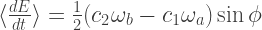
To check this, I numerically evaluated the ODEs above and calculated the expected growth curve, plotted below in yellow.

You can see that the agreement is excellent for this low growth rate, and at later times the oscillating solutions almost exactly follow the curve.

A second interesting thing is that the oscillators adjust their frequencies such that they are approximately out of phase. To see why this might occur, let’s examine growth of the total oscillator energy , i.e.

From the ODEs, we can do a bit of algebra to show that

If we assume that the oscillators are at their own natural frequencies, and that they are out of phase, then after a little more algebra we can take the time-average and show

Therefore, for maximum growth in energy and . Also, for both the same sign and the natural frequencies equal, there is no net growth in oscillator energy.

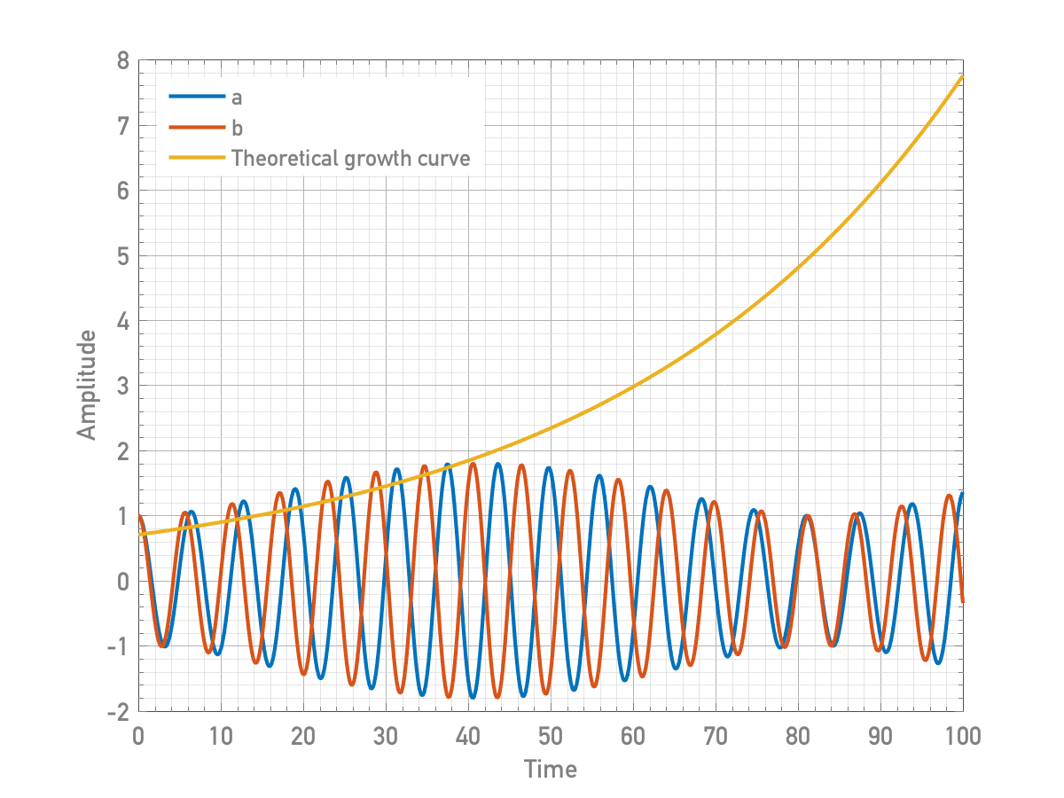
Finally there are some other secondary effects at play here. If the natural frequencies are different and the coupling not very strong, the growth doesn’t occur forever:

You can see that what’s happened is the oscillators have gotten out of a growing phase with respect to one another. They’d like to be at , but the fact that one would like to oscillate a bit more quickly means that they can’t sustain that relative phase difference forever.

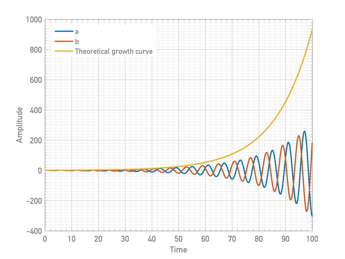
However, bump up the coupling a bit and the oscillators will happily stick at  even when their frequencies are different. The growth is so rapid that there’s no time for the oscillator to revert to it’s natural frequency, and so the oscillators are said to be ‘phase-locked’. Very roughly, this occurs when .

You might well wonder what the point of all of this is. My personal interest arises from plasma physics, where more or less everything reduces to an oscillation of some sort. One oscillator is the electron fluid, which oscillates at the plasma frequency . A second common oscillator is some form of electromagnetic wave at frequency . Typically these frequencies are very different, but can be coupled through the action of a third high-amplitude electromagnetic wave , commonly provided by a laser pulse. In this case the coupling strengths are proportional to the laser intensity and the density of the plasma. When the laser intensity is very large, all sorts of interesting nonlinear oscillator phenomena come into play. One example of which is Stimulated Raman Scattering (SRS) where a plasma resonantly scatters a laser pulse if .

The investigation of SRS in certain kinds of laser-plasma interactions formed a core of my PhD thesis so I thought it best to write a little about it, even tangentially, while I can claim a reason to.