Recently the extractor fan in my bathroom has started malfunctioning, occasionally grinding and stalling. The infuriating thing is that the grinding noise isn’t perfectly periodic – it is approximately so, but there are occasionally long gaps and the short gaps vary slightly. This lack of predictability makes the noise incredibly annoying, and hard to tune out. Before getting it fixed, I decided to investigate it a bit further.
The terminally curious may listen to the sound here:
https://www.dropbox.com/s/4xh1gmrjry10eky/FanSound.ts?dl=0
This was recorded from my phone, you can also hear me puttering around in the background.
After dumping the audio data, I looked at the waveform and realised it was quite difficult to extract the temporal locations of the grinding noises from the volume alone. As a good physicist I therefore had another look in the frequency domain, making a spectrogram.
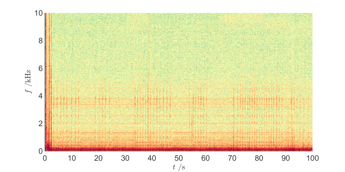
Every 200 ms I have taken a chunk of the waveform and computed the Fourier transform – the amplitude of this is plotted above as a function of time. You can see the occasional features lasting approximately 500 ms at around 2 – 4 kHz – this is exactly the annoying grinding sound. you can also see the infuriating random gaps between clusters of events, and within each cluster the periodicity isn’t exactly equal.
Integrating the spectral power between 2 and 5 kHz, I then have a time series of the noise signal:
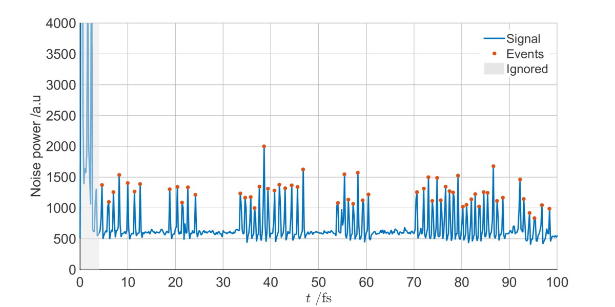
Having located the positions of the grinding noises, I can now do the analysis I wanted: finding the distribution of times between noises.
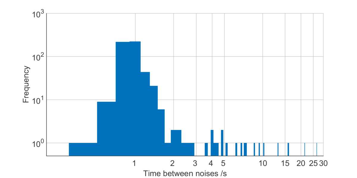
The quasi-periodic component has period 1 ± 0.24 seconds – almost periodic, but annoyingly not quite. There can also be longer gaps of up to 30 seconds between noises, adding to the annoyance. The fact that the mean period is very close to 1 second suggests an artificial reason for the noises – e.g. try to spin the fan up, if it fails, try again in 1 second.
This behaviour, intermittent regions of periodicity separated by gaps much longer than the characteristic time of the periodicity, looks very much like some simple chaotic systems, as suggested in the title.
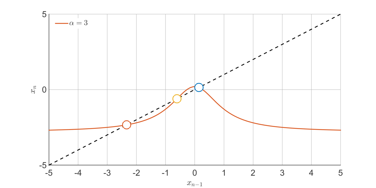
In particular, one can construct a 2D discrete mapping with separate fast and slow timescales – we’ll look at the Rulkov model built for irregularly bursting neurons as in e.g. here and here. The mapping is as follows:
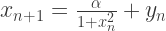
If you squint at the update equation for 


The other equation for 
Here 
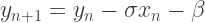
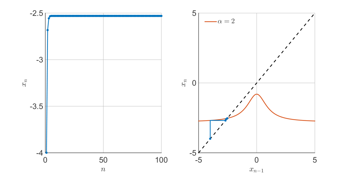
Raising
There is still only one fixed point, but
The transition is sudden – when
From above, the transition to chaos occurs when we go from 3 to 1 fixed point, i.e. the red and yellow points above merge into one. By fiddling with the mapping for long enough, it is possible to show that this happens at the points:

Plotting the fixed points of the mapping 
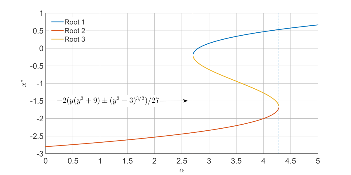
When 
So, this is all very interesting, but how does it compare to my extractor fan? As it turns out, pretty well:
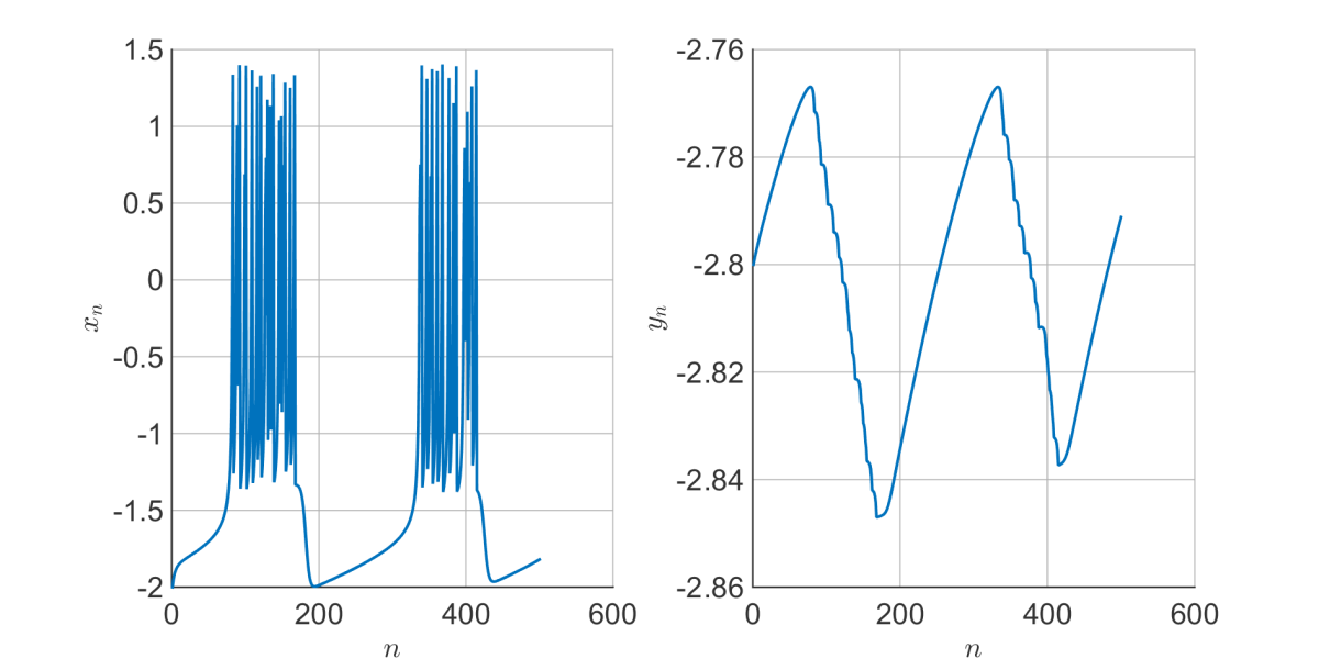
 , and is able to vary.
There are isolated bunches of spikes in
If we find the peaks in
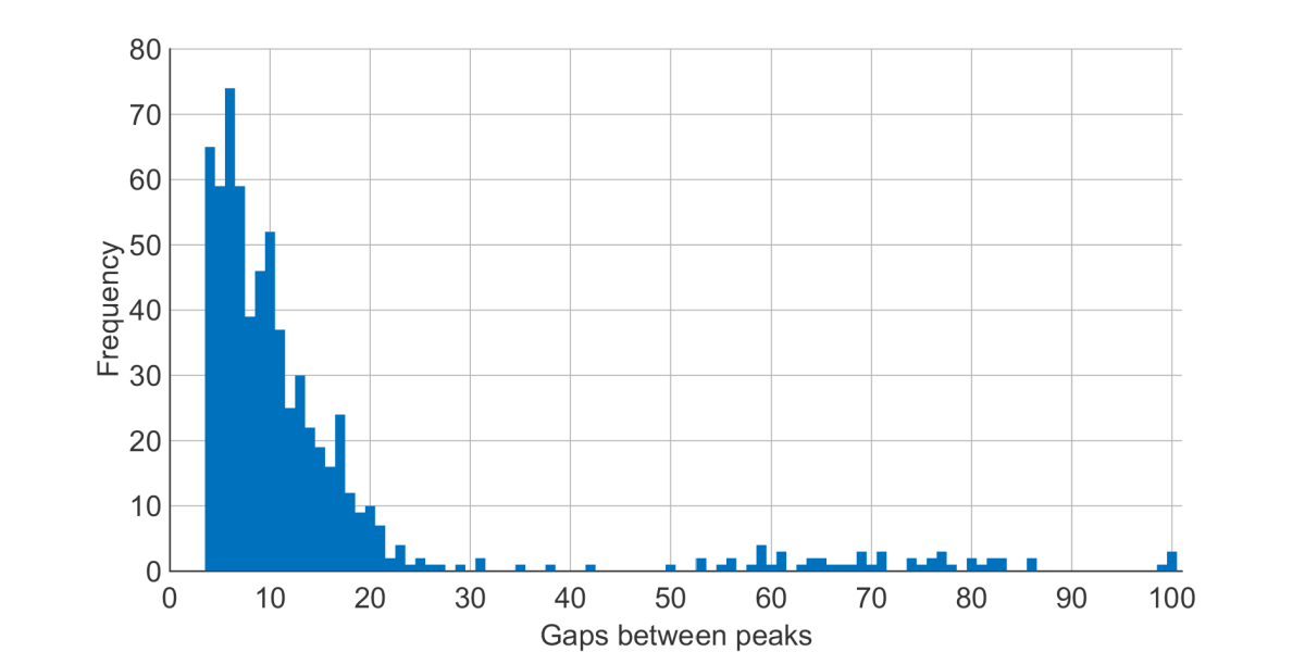 .
.Again, a broad quasi-periodic mass at small periods, and some scattered gaps at much longer periods. The similarity isn’t perfect, but it does suggest the same idea of timescale separation can explain my annoying extractor fan.
If you have an idea for a toy mechanical model which might also explain this phenomenon, get in touch!

Great analysis to get to the semi-stable chaotic model! We use a similar approach to your starting fourier transform for vibration analysis. But from there we jump to physical design characteristics to try to isolate which component is active at that frequency/harmonic, eg fan rpm, ball bearing diameters and rpm, AC power frequency.
LikeLike
Interesting. Do you have some kind of model which predicts resonant frequencies for different components?
LikeLike