Here’s a fun question – let’s consider, purely in the abstract, the notion of quickly putting on a lot of weight. If, hypothetically, one were to weigh themselves every day and, conceptually, throw away all of the results which showed an increase in weight, what, in a strictly Platonic sense, are the odds that actually they’re just a fat shit not actually losing any weight?
Simulation
Let’s engage in this fun thought experiment, as ridiculous as it may seem to the better amongst us who eat well and exercise regularly.
Suppose your real weight fluctuates about a mean 


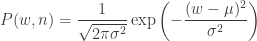
i.e. independent of 
Also suppose that you keep track of your weight, and only record a measurement when it is below your previous record low weight. A sequence of measurements may then look like this, monotonically decreasing:

Here we’ve simulated the measurement process – every day, draw a sample from 
It is, sadly, a lie. Here it is overlaid on many similar simulations and their average:

The trend is clearly a rapid initial ‘fall’, followed by an increasingly slow decline – intriguingly similar to the expected weight-loss profile if you were actually caring about your body.
Let’s think about how to model this process in a couple of ways.
Method 1: Iterated expectation
Starting from the beginning, on day 1 the expected value of the measured weight is just (handwaving the integral limits away):

Easy enough. What about day 2? This is more interesting – the probability of the actual weight stays the same, but not the reported measurement – the latter is clamped at a maximum of 

The particularly eager reader can confirm that this evaluates to

where the error function 
Each day’s measurement is then a function of the previous days – hence ‘iterated expectation’. Let’s see what this looks like compared to the simulation:
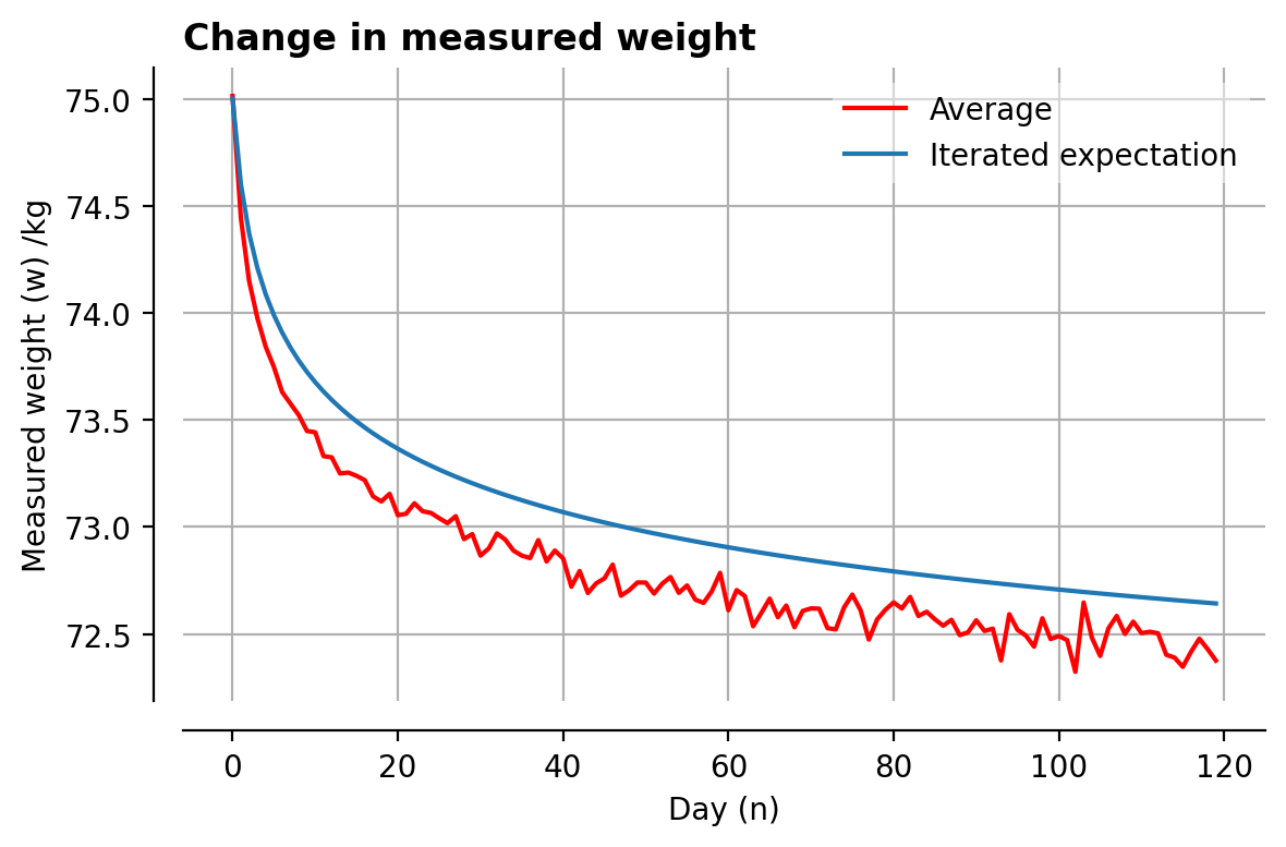
It’s not terrible, but it’s not perfect either. The general shape is right, and it might converge to a similar value, but we can do better.
Method 2: Expected minimum
There is another, simpler, way to look at this problem: after
As the distribution of our measurements is constant over time – it exhibits homoscedasticity – for each day is there is a certain probability of measuring a value under 

where 


We’re interested in the conjugate case, where 

The probability density distribution of the minimum measured value after
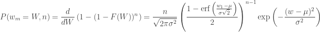
Phew. We’re not quite there – to get the expected value, we need to integrate this expression again. Unfortunately there’s not a closed form (as far as I can tell), but we can still do it numerically:

Bang on! Well done us.
Method 3: Obscure Stack Exchanging
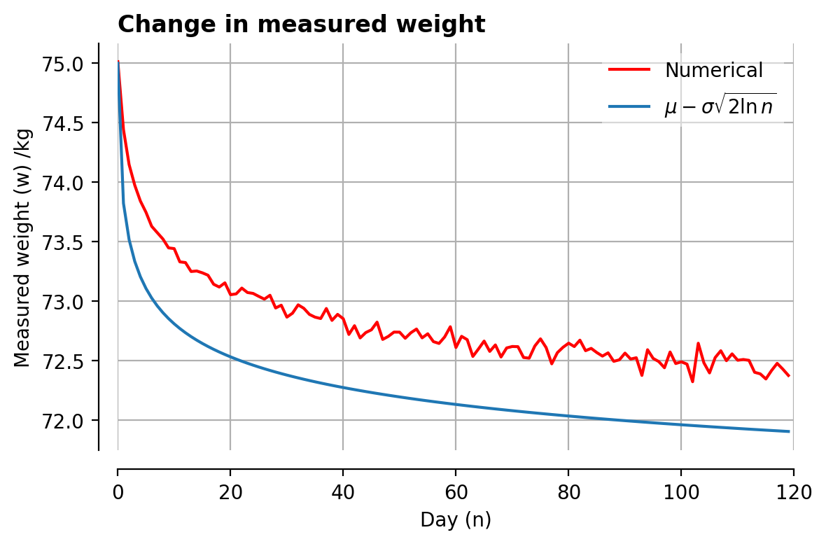
The final method is to go spelunking into the dusty corners of the internet. This comment suggests that a simple approximation is:

Plotting it out, it isn’t too bad! Points to whoever can derive it for me:
And finally, a comparison of all methods:

…so?
Although the last method results in the worst approximation, it probably represents a good rule of thumb for figuring out if you’ve actually lost weight:
- Days 1-10: calculate the mean and standard deviation of your natural weight by measuring it properly every day.
- Days 10-99: diet, don’t diet, who cares – just keep a record of your minimum weight so far. We all know careful record keeping is better for the body than any amount of quinoa anyway.
- Day 100: after 90 days,
(yep, 4 nines!), so if you are 3 or more standard deviations below your starting weight, you’ve probably smashed it. Well done! Celebrate by doing some more maths.

Cool post!! I never thought about it haha, I guess the same can be said from the other perspective, ie: you only record your maximum weight instead of the minimum. So maybe I’m not getting fat, it’s just a statistical artefact 🙂
I have a question about your method. Which $\sigma$ did you choose for your distribution? I guess the results depend a lot on that since a bigger sigma would make the illusion of losing/winning weight faster.
LikeLike