Damp and Driven Swingers

We’ll continue the theme of this fledgling blog along the lines of fractals, pretty pictures, spirals and Matlab. All of this neatly encapsulated in the concept of the damped and driven oscillator, alluded to somewhat scandalously in the title. In particular, for simplest conceptualisation (and maximum innuendo potential) we’ll look at the humble pendulum.

The setup is simple and sketched below. We have a particle of mass $m$ mounted on a light rigid rod of length $l$ . The only force acting (for now) is gravity, pulling the particle vertically downwards with a force $mg$ . If the pendulum is currently swinging out at angle $\theta$ , there is then a torque acting to swing the pendulum downwards of magnitude $l \times mg\sin\theta$ – the force perpendicular to the rod multiplied by the distance to the pivot.

The rotational equivalent to Newton’s law is

$\tau = I\ddot{\theta}$

where $\tau$ is the applied torque, $I$ the moment of inertia and $\ddot{\theta}$ the angular acceleration experienced by the particle. Substituting everything in we have

$\ddot{\theta} = -\frac{g}{l}\sin\theta \rightarrow \sin\theta$

where for convenience we ignore the $g/l$ factor. This is equivalent to changing the length of the pendulum such that the frequency is 1 radian/second, and doesn’t affect the subsequent analysis. This equation as it stands can’t be solved using elementary functions (we need elliptic integrals), so for our purposes isn’t very interesting. If we take $\theta$ very small such that $\sin\theta \approx \theta$ then there is a solution, namely $\theta(t) = \sin(t)$ , which again isn’t hugely interesting and doesn’t make any pretty pictures.

Instead, we’ll look at understanding the behaviour of the pendulum in a different way. Usually we look at paths the pendulum traces in the time domain, that is the plane defined by the coordinates $(t,\theta)$ . There we will see a simple sin wave which is nice and simple to describe. We can also plot out paths using the coordinates one level higher $(\theta, \dot{\theta})$ – the instantaneous angles and angular velocities of the pendulum (often called phase space). This is more interesting because we can actually get some answers without resorting to a small angle approximation, allowing us to explore a wider range of behaviour.

Set $\omega \equiv \dot{\theta}$ , then we have the two equations

$\dot{\omega} = -\sin\theta$

$\dot{\theta} = \omega$

and as we did before with the ants, we can combine these two to relate $\omega$ and $\theta$

$\frac{d\omega}{d\theta} = \frac{\dot{\omega}}{\dot{\theta}} = -\frac{\sin{\theta}}{\omega}$ .

This is nice because it’s a simple separable differential equation much like the ant problem, and we can solve away

$\int \omega d\omega = -\int \sin\theta d\theta$

$\frac{1}{2}\omega^2 = \cos\theta + C$

$\omega = \sqrt{2\cos\theta + C}$ .

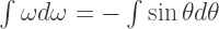
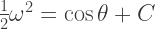
The integration constant $C$ parameterises the different solutions of our dynamical system, so it is important we know what it is. As a physicist, hearing the word constant should instantly point your agile mind towards constants of motion, the most obvious being the energy of the system. Here the instantaneous energy of the pendulum is composed of potential and gravitational energy and is

$E = mgh + \frac{1}{2}I\omega^2$

where $h = l(1 - \cos\theta)$ is the height of the pendulum from its resting position. We’ve taken $l = g$ , so if our initial conditions for the pendulum correspond to position and velocity $(\theta_0, \omega_0)$ , then the initial energy

$E_0 = mg^2(1 - \cos\theta_0 + \omega_0^2/2)$ .

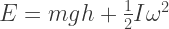
and we can see that our constant is related to the initial energy of the system as

$C = 2\left(\frac{E_0}{mg^2} - 1\right)$ .

This is important – as the starting energy changes, the type of solution we get in phase space qualitatively changes. We can also note that the time derivative of the energy

$\dot{E} = mg^2(\sin\theta\dot{\theta} + \dot{\omega}\omega) = 0$

where we’ve used our initial equation of motion to substitute in for $\dot{\omega}$ . As the energy doesn’t change, the pendulum always sits on the same class of solution as it wanders through phase space – this is an important point we’ll come back to later.

For starters, lets examine the motion of a low-amplitude oscillation. That is a low total energy, and $\theta \ll 1$ . In this case $\cos\theta \approx 1 - \theta^2/2$ and so $\omega^2 + \theta^2 = E_0/mg^2$ . In phase space then the pendulum should trace out a circle with a radius proportional to the square root of the total energy.

In the above animation I’ve evolved the differential equations in time directly to get both the pictures in real space and phase space simultaneously. The fact that the radius of the circle traced in phase space stays constant means the energy of the system is being conserved, which is what we want to see and is a good check that things are working as expected.

We can also increase the initial energy of our pendulum above the ‘escape velocity’ which will allow it to spin all the way round, and the picture in phase space looks very different.

We can look at all of this together by plotting out the different trajectories according to the formula we derived earlier.

For low-energy starting conditions we end up with a circle as before – this requires approximately $E_0/mg^2 < 0.5$ , and means that the pendulum can’t start too high up or swinging too quickly. As the energy increases the circle spreads out, and this corresponds to the pendulum getting close to being upside down. It spends more time up there as a perfect upside-down state would in fact be an (unstable) equilibrium position. If the energy were exactly $E_0/mg^2 = 2$ the pendulum would swing round and stop perfectly balanced at the top – this is the purple line above. Slightly more energetic and the pendulum can escape the bounds of its boring circular orbits and spin freely – these are the lines above and below the ‘eye’. The two types of motion are qualitatively different, even though they’re described by the same equation, and the purple line separating them is known (somewhat unimaginatively) as the separatrix. Our dynamical system keeps its starting energy – it is non-dissipative – and so if the pendulum begins inside or outside the separatrix it stays there forever, whirling away.

This doesn’t sound like very much fun, so lets have a go at modelling something a little more like the real world. Specifically we should introduce some dissipation into the system, a way of losing energy to the outside world. The simplest thing to do is stick a term into the differential equation that accelerates the pendulum in the opposite direction, i.e. slowing it down. Make this term proportional to the velocity of the pendulum and the equation becomes

$\dot{\omega} = -\sin\theta - q\omega$

where $q$ is a measure of how quickly the pendulum slows down. We can again look at the rate of change of energy of the system and find

$\dot{E} = -mg^2\omega^2q$

so energy is dumped off into the surroundings at a rate proportional to $q$ and the square of the angular velocity. This means in phase space our pendulum will be drifting between paths we plotted above as the energy decreases, and so should spiral into the middle.

Now we’ve come across spirals in this blog before, so with our newfound knowledge lets see if we can get to the bottom of this one. It looks a little funkier but that just adds to the fun. As a good scientist I’ll gratefully note the assistance of the paper ‘A look at damped harmonic oscillators through the phase plane’ by Daneshbod et al, you can find the paper and other details here http://teamat.oxfordjournals.org/content/30/2/62.abstract.

Unfortunately this problem is a little trickier so we’ll need to resort to the small angle approximation that $\sin\theta \approx \theta$ , and we have

$\frac{d\omega}{d\theta} = -\frac{\theta}{\omega} - q$ .

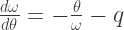
This equation isn’t separable anymore thanks to that damping term messing up the right hand side, so we’ll make the substitution $y = \omega/\theta$ which means

$\frac{d\omega}{d\theta} = \theta\frac{dy}{d\theta} + \frac{\omega}{\theta}$

and the equation turns into something nice and separable (though not necessarily simple)

$\frac{y}{1 + y^2 - qy}\frac{dy}{d\theta} = -\frac{1}{\theta}$ .

The left hand side is a bit nasty, but we can get it into a simpler form by making the substitution $x = y - q/2$ to remove the term linear in $y$ on the bottom. The resulting integral is easy enough to evaluate and we have

$\frac{1}{2}\ln\left(\frac{\omega^2}{\theta^2} - \frac{q\omega}{\theta} + 1\right) + \frac{q}{\sqrt{4 - q^2}}\tan^{-1}\left(\frac{\frac{2\omega}{\theta} - q}{\sqrt{4 - q^2}}\right) = -\ln K\theta$

with some integration constant $K$ taken inside the logarithm. Taking $q \rightarrow 0$ we return to the equation of the undamped pendulum as we should, which is a nice indication that our algebra has been ok so far! This way we can also equate $K = E_0/mg^2$ . This is lovely, but not yet obviously the equation for a spiral. At this point I needed a hint which the paper referenced above was kind enough to provide. We can cunningly make the substitutions

$u = \omega - \frac{q\theta}{2}$

$v = \theta\sqrt{1 - \frac{q^2}{4}}$

and the complex expression becomes

$\ln(u^2 + v^2) + \frac{2q}{\sqrt{4 - q^2}}\tan^{-1}\left(\frac{u}{v}\right) = 2\ln K$ .

Finally if, as that equation is screaming out for, we switch to polar coordinates

$u = \rho\sin\phi, \quad v = \rho\cos\phi$

we have

$\ln\rho + \frac{2q}{\sqrt{4 - q^2}}\phi = \ln K$

which becomes upon exponentiation

$\rho = Ke^{-p\phi}, \quad p =\frac{q}{\sqrt{4 - q^2}}$ .

So finally, our favourite logarithmic spiral makes a return. The speed at which we spiral into the centre in phase space increases with the damping rate as expected, but shoots up very quickly near $q = 2$ . This corresponds to the pendulum approaching a critical damping rate, and marks a qualitative change in behaviour from gradually shrinking oscillations to a single swing. Above this point there is no spiral in phase space, rather a straight line towards the origin.

So we’ve done some maths, we’ve made some plots, and we’ve even found a logarithmic spiral hiding amongst the noise. What about the pretty pictures I promised? For this there is a final ingredient to add to the picture – a driving term in the equation of motion. If we add an oscillating torque to the damped pendulum it will never slow down to zero, the input torque is always adding energy to the system, and the equation of motion looks like

$\dot{\omega} = -\sin\theta - q\omega + F\sin\Omega t$

where $F$ and $\Omega$ define the amplitude and frequency of the torque. This equation is well known to be chaotic, that is the long-term behaviour of the pendulum is exponentially sensitive to the initial conditions. In the pictures below I have created a plane of initial conditions, angles and velocities, and coloured each point depending on where the pendulum ends up after 20 seconds of motion.

In the animation below I slowly turn up the amplitude of the driving force. When small, the plane is smoothly coloured which means that as we try different initial conditions the pendulum ends up in similar places, and if the initial condition changes slightly the final position also changes slightly.

As the forcing increases the plane gets messy and torn up. This marks a transition to chaos where only a slight change in initial conditions leads to drastically different long-term behaviour.

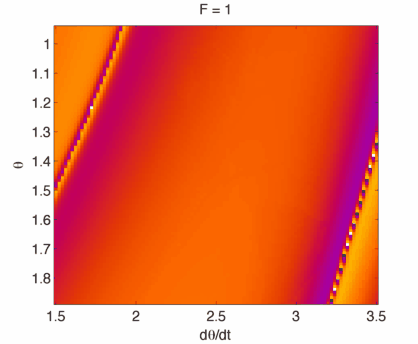
We saw this kind of transition in the logistic map a few posts ago, but there we also saw the existence of ‘islands of stability’ deep into the chaotic region where a semblance of normality briefly returns. With enough poking around we can see similar phenomena here. In the higher-resolution plot below there is a literal island of stability, where the colours are relatively smooth and aren’t changing by huge amounts. There is also a hint of a characteristic chaotic ‘stretching and folding’ of the plane, or in this case a light whisking of the plane perhaps.

The humble single pendulum often loses out to its sexier and livelier older brother, the double pendulum, but hopefully I’ve convinced you of the beginnings of beauty there, deep in the melange.

Almost looks like work

Damp and Driven Swingers

Leave a comment Cancel reply

Share this:

Related

Leave a comment Cancel reply