A few posts back I was concerned with optimising the WiFi reception in my flat, and I chose a simple method for calculating the distribution of electromagnetic intensity. I casually mentioned that I really should be doing things more rigorously by solving the Helmholtz equation, but then didn’t. Well, spurred on by a shocking amount of spare time, I’ve given it a go here.
UPDATE: Web app now available, check it out at https://wifi-solver.com
The Helmholtz equation is used in the modelling of the propagation of electromagnetic waves. More precisely, if the time-dependence of an electromagnetic wave can be assumed to be of the form 


where 


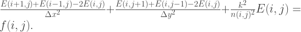
This is a linear equation in the ‘current’ cell 


This is slightly tricky due to the fact that a 2D labelling system 


A pair of cells 


The row in the matrix equation corresponding to the

where there are 


Fortunately this problem has crept up on people cleverer than I, and they invented the concept of the sparse matrix, or a matrix filled mostly with zeros. We can visualise the structure of our matrix using the handy Matlab function spy – as plotted below it shows which elements of the matrix are nonzero.

Here 
Moving on to the physics then, what does a solution of the Helmholtz equation look like? On the unit square for large 
In this calculation I’ve set boundary conditions that 
Visualised below are a selected few pretty pictures where I’ve taken a logarithmic colour scale to highlight the positions of zero electric field – the ‘nodes’. As the animation proceeds

Once again physics has turned out unexpectedly pretty and distracted me away from my goal, and this post becomes a microcosm of the entire concept of the blog…
Moving onwards, I’ll recap the layout of the flat where I’m hoping to improve the signal reaching my computer from my WiFi router:

I can use this image to act as a refractive index map – walls are very high refractive index, and empty space has a refractive index of 1. I then set up the WiFi antenna as a small radiation source hidden away somewhat uselessly in the corner. Starting with a radiation wavelength of 10 cm, I end up with an electromagnetic intensity map which looks like this:

This is, well, surprisingly great to look at, but is very much unexpected. I would have expected to see some region of ‘brightness’ around the electromagnetic source, fading away into the distance perhaps with some funky diffraction effects going on. Instead we get a wispy structure with filaments of strong field strength snaking their way around. There are noticeable black spots too, recognisable to anyone who’s shifted position in a chair and having their phone conversation dropped.
What if we stuck the router in the kitchen?

This seems to help the reception in all of the flat except the bedrooms, though we would have to deal with lightning striking the cupboard under the stairs it seems.
What about smack bang in the middle of the flat?

Thats more like it! Tendrils of internet goodness can get everywhere, even into the bathroom where no one at all occasionally reads BBC News with numb legs. Unfortunately this is probably not a viable option.
Actually the distribution of field strength seems extremely sensitive to every parameter, be it the position of the router, the wavelength of the radiation, or the refractive index of the front door. This probably requires some averaging over parameters or grid convergence scan, but given it takes this laptop 10 minutes or so to conjure up each of the above images, that’s probably out of the question for now.
UPDATE
As suggested by a helpful commenter, I tried adding in an imaginary component of the refractive index for the walls, taken from here. This allows for some absorption in the concrete, and stops the perfect reflections forming a standing wave which almost perfectly cancels everything out. The results look like something I would actually expect:
END UPDATE
It’s quite surprising that the final results should be so sensitive, but given we’re performing a matrix inversion in the solution, the field strength at every position depends on the field strength at every other position. This might seem to be invoking some sort of non-local interaction of the electromagnetic field, but actually its just due to the way we’ve decided to solve the problem.
The Helmholtz equation implicitly assumes a solution independent of time, other than a sinusoidal oscillation. What we end up with is then a system at equilibrium, oscillating back and forth as a trapped standing wave. In effect the antenna has been switched on for an infinite amount of time and all possible reflections, refractions, transmissions etc. have been allowed to happen. There is certainly enough time for all parts of the flat to affect every other part of the flat then, and ‘non-locality’ isn’t an issue. In a practical sense, after a second the electromagnetic waves have had time to zip around the place billions of times and so equilibrium happens extremely quickly.
Now it’s all very well and good to chat about this so glibly, because we’re all physicists and 90% of the time we’re rationalising away difficult-to-do things as ‘obvious’ or ‘trivial’ to avoid doing any work. Unfortunately for me the point of this blog is to do lots of work in my spare time while avoiding doing anything actually useful, so lets see if we can’t have a go at the time-dependent problem. Once we start reintroducing 
This is exactly what the FDTD technique achieves – Finite Difference Time Domain. The FD means we’re solving equations on a grid, and the TD just makes it all a bit harder. To be specific there is a simple algorithm to march Maxwell’s equations forwards in time, namely

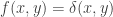
I’ve introduced a current source 


With the router in approximately the correct place, you can see the radiation initially stream out of the router. There are a few reflections at first, but once the flat has been filled with field it becomes static quite quickly, and settles into an oscillating standing wave. This looks very much like the ‘infinite time’ Helmholtz solution above, albeit at a longer wavelength, and justifies some of the hand-waving ‘intuition’ I tried to fool you with.

Hey! Nice simulation, here is a numerical suggestion. Instead of computing M^{-1} and multiplying, you can solve ME=f directly by using a linear-systems-of-equation solver. It avoids calculating the inverse!
LikeLiked by 1 person
I’ve been pointed to lsolve() in Matlab, I’ll give it a go and hopefully things will speed up nicely. Cheers.
LikeLike
There is a small mistake in the translation from the 2D labeling system to the 1D system, it should be n = M(i-1) + j instead of (M-1)i + j. This way the mapping (N,M) -> NM actually works
LikeLiked by 2 people
Good spot! Thanks, I’ll update.
LikeLike
Great article! Please make a web service out of that, where one can draw the walls and have the optimal router position computed!
LikeLiked by 2 people
Thanks! That would be excellent, but perhaps unfeasible at the moment. While it makes nice pictures, the code as it stands doesn’t use accurate values for the different refractive indicies of walls, windows, doors etc. It’s also only 2D and doesn’t include the full spectrum of the WiFi radiation. For a full model I suspect these things would have to be included, but who knows, perhaps I should experimentally map the field strength myself and see how accurate this is?
That’s for another time though…
LikeLike
Please please please do this. This is a service you could sell to businesses! Have a set of 4 different generic surface types (plaster wall, brick/concrete, glass, wood) and you can probably find details of their effect on electromagnetic radiation online already.
My office has 25 access points, placed with guestimation and there are plenty of dark spots! This would really help us improve our guestimations!
LikeLiked by 1 person
I’ve just done some rudimentary analysis for kicks due to me not being able to explain to my now former office suite landlord in any way possible that 800ft^2 of coverage, between old impenetrable red brick walls, off a 2.4ghz 802.11n router, with an antediluvian dedicated 7mbps DSL connection, for 15-20 devices–yes, this is something that even I cannot “fix”.
I will say this, however, and that is I was able to stream 1080P 30sec clip off youtube on two devices simultaneously. I rewired the RJ-11 plug and fit the wall with a cat jack, split the neighboring suites RG-6 that had a piping hot 7mbps dedicated broadband line. then used SSTP/SFTP cat6a cable to the router. So I sort of committed a crime but i think you get my point–there’s limitations in data transmission and in the realm of network alchemy we’ve yet to turn bonded DSL into an optical signal.
Now i’d be curious to see if you’d get any improvements using this cable from your modem to the router. I’ve not done any packet analysis (i have a life sort of) but holy smokes this stuff was like $250 for a 1000′ spool and I’m currently running this crap all over my house because the performance increase in high interference areas was visibly evident compared to a non SFTP ordinary cat5e. lightyears better than the phone line that was going into the same router. something to mull on. what a lot of people neglect to understand is their goddamned wireless peripherals (logitech especially) can cause more timeouts, dropped connections, and general data connectivity pademonium. But yeah this post is fresh2death. And yeah it almost does look like work.
LikeLike
Interesting to see the mathematics used to calculate optimal placement. There are many free programs that will dynamically map RSSI, SNR and interference to floor plans which give you a realtime view of coverage. Example; wifi explorer, wifi analyzer, Xirrus Wi-Fi Inspector, any Cisco Meraki wireless access point
LikeLike
Would the waves permeate through doors but not walls? I feel like basing this off reflections from walls only and no wall permeability is a bit rough. In saying that I think this is fantastic!
LikeLike
This is all rather rough, mainly meant as a proof of principle. At the moment I’m reading in refractive index values from a bitmap for the grid, it should be pretty simple to add in some varying permeability by ‘painting’ the doors/windows etc. a different shade of gray. Thanks for the comment.
LikeLike
Please please please do this. This is a service you could sell to businesses! Have a set of 4 different generic surface types (plaster wall, brick/concrete, glass, wood) and you can probably find details of their effect on electromagnetic radiation online already.
My office has 25 access points, placed with guestimation and there are plenty of dark spots! This would really help us improve our guestimations!
LikeLiked by 1 person
it already exists, Arubanetworks has a product called visualRF that does just this
LikeLike
Thanks for the tip
LikeLike
As does Aerohive
LikeLike
first!
LikeLike
While very interesting, it misses extra variables other than just permeability of walls and refraction values. The presence of other wireless radios on the same or similar frequencies are not even accounted for or other sources of interference. Without accounting for your neighbors wifi colliding and canceling out your own signal it could never be used for business deployment or home at that matter. Not to mention your own access point placed too close to another on the same channel can cause interference as well and would have to be accounted for in these equations.
LikeLike
This is pretty cool! Could you publish your code?
LikeLiked by 1 person
It’s a bit of a mess at the moment, but sure once it’s cleaned up a bit.
LikeLiked by 1 person
Seems that Mathworks has included the capability whereby Matlab code can be spat out as C, leading to the possibility of a smartphone app for data collection about positions of objects (and possibly, signal-strength data collection that could help estimation of parameters such as transmissivity), even, perhaps computation of the paths themselves, as recent devices have some killer math capabilities.
It also makes me wonder whether circularly-polarized signals, since antennas for it naturally ignore the first reflection, wouldn’t be much better for work in the type of tortured space we live in.
Finally, MIMO would seem to be no better at covering genuinely dead spots, but could goose up signal levels in marginal areas, making all this mostly academic. Have you had experience with it?
LikeLike
The code is simple enough to write in C, I just worry that inverting a large matrix will eat up too much RAM – it spikes to a few GB on my laptop. I’m experimenting with iterative methods which are much less memory hungry, or maybe representing the matrix in block diagonal form, in which case the inverse can be computed ‘piecewise’.
Unfortunately I’m not an expert on this so I can’t really comment on the practical side, but its been interesting to come into contact with people who are. Cheers.
LikeLike
That would be awesome. I’m currently building a house, and I’ve planned the location of my router, but I’d love to see if it’s optimal or not, so I can change it before I run the cables 🙂
LikeLike
If you start a github project, maybe someone will help too? or at least test it further
LikeLiked by 1 person
I’d like to see the code as well
LikeLiked by 1 person
Yep, looking forward to your code on GitHub
LikeLike
The images / sensitivity indicate that you have high-Q resonances, so probably the refractive index for the walls is too high. They are probably much closer to 1, with a small imaginary component, than the first model.
LikeLiked by 1 person
Thanks, I’ll try that. I must admit, I forgot that I could include absorption in the walls with a complex refractive index.
LikeLike
I think that’s the key. From here:
Click to access 1998_EM%20properties%20of%20concrete%20at%20microwave%20freq%20range_HCR%20&%20OB.pdf
I plugged in some actually sensible values and things look much more reasonable. Thanks!
LikeLike
Could you post the references to the applications / scripts / documentation you used in order to write this great post ?
Thank you !
LikeLike
Hi Stefan, I wrote the script in Matlab, I’ll consider posting it once cleaned up a bit. As for documentation, well that just came from my rapidly fading undergraduate physics I’m afraid. The mathematical and computational techniques are very standard and will be documented thoroughly in any numerical methods textbook.
LikeLiked by 1 person
Thank you, and for the update ! Btw, I’m an android / ios developer. Don’t hesitate to contact me if you need something.
LikeLike
Absolutely amazing work. My company works on Wi-Fi engineering and deployments. While we have tools that provide heat maps, I think there would be much more value in having a tool that shows RF behavior. I would be interested to see the same simulation with multiple AP’s and perhaps at 5 GHz. Brilliant!!!!!
LikeLike
>More precisely, if the time-dependence of an electromagnetic wave can be assumed to be of the form sin(wt)
I think here you make a serious mistake. It implies that the time phase is uniform in the apartment. The standard implication is that the time dependence is exp(Iwt) and you search for a complex E(x) solution.
LikeLike
Apologies, I intended to write the article for a layman audience and so avoided complex numbers at the beginning. Of course, then I couldn’t help myself and a did a bit more maths throughout. What I actually did was, as you suggest, assume factorisation of e^{iwt) and solve for complex E(x,y).
LikeLike
If you’re interested in exploring other ways to solve this problem, I’d suggest rewriting your problem in block matrix notation. You should end up with a block tridigonal problem. The “big dimension” ends up being trivial to solve using e.g. Gaussian elimination. The “block matrix” elements are non-sparse, and so can be solved efficiently using ordinary Matlab matrix notation.
This might be a useful resource for explaining that.
LikeLike
Thanks for the suggestion, my numerical methods aren’t quite up to scratch and this is something I’ve read about but never implemented. I’ll have a look!
LikeLike
I would suggest doing some experiments with your receiver by arranging according to the numerical result. How good is the agreement?
LikeLike
I’m not at my flat right now, but that would be very interesting! There’s also some evidence that the orientation of the receiving antenna matters quite a bit, perhaps motivating a full 3D approach.
LikeLike
I would consider an antenna oriented perfectly vertical. 3D approach would mean calculations so long you will have changed furniture by then.
Also, your calculations are very nice (the idea, I haven’t checked the physics) but keep in mind another (maybe even more important) element: other networks.
Of course they affect especially the placement of the receiver and not the placement of the emitter, but still it’s worth mentioning it somewhere.
LikeLike
Very interesting work. However I suspect that your assumption of a sine wave is strongly overestimating the interferences pattern (seen in radial direction around the source due to the wave reflected by the not-so-absorbing nearest wall). The actual wifi signal is phase modulated and so i believe that mostly the direct “time of flight” signal between the emitter and the receptor needs to be considered. The “wifi signal” won’t be necessary be the one with the highest amplitude but the one with the correct phase shift sequence. I am not an engineer but only physicist… so i guess the actual data processing is much more elaborated than that but a signal with a variable phase shift will not have such strong interferences patterns. Moreover concrete is relatively transparent to microwaves. Worth some more thinking !
LikeLike
I don’t know that you could really calculate it, but polarization will have a lot to do with your signal strength at the computer. If the antennas are cross polarized with the received signal you can lose ~3dB all other things being equal. Might be fun for another day?
LikeLike
I just fold a piece of kitchen foil, shiny side as reflective surface, in the entrance of areas that have low wifi signal and bounce it just a little further, round corners etc. no calculations just a bit of guestimate/common sense in relation to the path the wifi signal travels from the router to where I need more signal. Works fine for me and can be used as a temporary or a permanant solution as required.
LikeLike
great job! perhaps you could try 3D. it’ll be interesting to know how the outcome is like.
LikeLike
Im studying to be an engineer right now and these complex calculations are amazing!! You guys sound awesome in your comments. I cant wait to become an engineer!. This is motivation haha.
LikeLike
http://www.overclockers.com.au/
led me to this blog.
Using “Wifi Manager” (Android), I could measure real-time signal strengths.
It varies as well, by:
1) orientation of the receiver’s aerial (my smartphone) as an angle, or front-back-side orientation, relative to the transmitter’s aerials.
2) if any metal objects (earthed, powered, or not?) are in the surfaces between the two aerials.
3) the “amount” of mass between the two aerials; one “innocent” wall totally parallel to the two aerials is the biggest block (no air spaces!)
4) brand & type of transmitter; discovered when my wireless-router-modem needed replacing.
From Australia …
LikeLike
Great – but I think this would be fairly easy to simulate for those that have access to and skills in Comsol Multiphysics http://www.comsol.se/comsol-multiphysics
LikeLike
Yes definitely, I’m well aware tools exist for this, it was really just for a bit of fun! Had I known the interest this would generate I would have put a disclaimer at the top.
LikeLike
Helmholtz? That thing looks like the millennium simulation…
LikeLike
Hmm, my calculus skills are not that great (though I am a professional programmer, go figure). Anyway, I am really tempted to try turning this into into a computer algorithm that is run in Python, Ruby, or Go just to make it so that anyone can run it on their home setup.
I just need to figure out the best way to make this into an algorithm in my computer (again, the calculus is weak with me). Complex computational math is not something I have ever really tried.
LikeLike
Great work. Now take the whole thing and make it comprehensible to a mildly numerate psychologist .As regards WiFi placement I should avoid intervening walls and put the transmitter in a central position for greatest coverage? And never waste time on BBC online? Have you a mnemonic for all that? (Great stuff).
LikeLike
Hi I am physicist and would like to know in details of your method. Mind to share the calculation for both methods?
LikeLike
I’m interested to take a look at the code. Any samples on GitHub?
LikeLike
Cool, you should make a software for it 😉
LikeLike
How about Open EMS?
http://openems.de/start/index.php
LikeLike
I’m aware there are many open and closed source implementations for this sort of thing, it was mainly a bit of fun! Thanks for the link though, I’ll take a look.
LikeLike
Please, PLEASE either release this as a service. Even in an imperfect state (no accounting for windows, 2d only, etc) this would be extremely handy, not to mention just awesome to look at. Or release the source code so other people can have fun with it and develop it into something.
LikeLike
I love this post! Thank you!! I want to get my maths & physics books back out again! 🙂
LikeLike
Thanks! You definitely should
LikeLiked by 1 person
Why do you assume the radiation pattern of the router is perfectly omni-directional? Perhaps try fining some documentation regarding common antennas used for 2.4GHz and 5GHz ISM bands and simulate with different common radiation patterns?
LikeLike
Simplicity! The FDTD simulation used a simple linear antenna sticking out of the plane. This produces an omnidirectional radiation field, to simulate something more complicated I’d need to manufacture a more complicated antenna, which is where my knowledge runs out.
LikeLike
Ahh, okay. I just happen to be an RF engineer 😉
Common 2.4GHz antennas have silly radiation patterns that seem rather illogical even though they claim they are “omni-directional” (and on 2d representations this appears to be the case). Take this radiation pattern from the Monopole Antenna wiki page for example: http://upload.wikimedia.org/wikipedia/commons/2/20/Vpol_dual_band_blade_antenna_blade_L1_3D.jpg
LikeLike
Thanks for the link. As I’m assuming 2D symmetry, I’m effectively simulating an infinitely long dipole antenna. In order to visualise the radiation pattern more easily, perhaps I’ll implement a way to plot to Poynting vector as well as the fields. Cheers.
LikeLike
Have you considered accounting for the effect of electrical interference caused by appliances and mains power lines. In my personal experience I have seen significant signal drop caused by the mains power line going to the breaker box in my parents’ house (the breaker box was directly between my computer and the router, and moving a few feet left or right of the box would double my signal). Additionally, flat panel TVs, and bathroom mirrors block a lot of wifi signal because they are very large reflectors.
LikeLike
Thank you
Blog fantastic
Good luck
………………..
http://www.8ii.in
LikeLike
nice work you got there..
i’m myself an electric engineer who did something similar this course on my third year, i can share with you my code on matlab,its not precisely for wifi router but rather RF signals (100MHz to a few Ghz) but could work if adjusted properly.
in addition it has a gaussian source so it is more of an large distance radio transmition simulator.
have fun
http://www.megafileupload.com/en/file/561961/wave-propogation-project-rar.html
LikeLike
Thanks! As I’m sure you noticed, nothing I’ve done here is particularly different, the trick is obviously choosing the correct Matlab colourmap 😉
LikeLike
and a whole different approach to solve the helmholtz equation with paraxial direction approximation,but yea,similar idea.
quite weird that i’m the first to publish my code in here…as if i walking on the steps of giants in the middle of my Undergraduate degree 🙂
any fun ideas about what can i improve\try to do with my code?
LikeLike
Actually it’s interesting, I happen to have written my own SSPE-type simulation for modelling the propagation of laser pulses through plasmas. That’s on femtosecond and micron scales, so it’s interesting to see it applied in a completely different context!
LikeLike
i’m amazed that there are actually clocks that work in the femtosecond scale.
and here,as an EE i’m sticking to Khz and Mhz for my projects
LikeLike
Amazing Work!
You’r in top on the Russian PDA site 🙂
Thank you, Jason.
LikeLike
Hello Russia!
LikeLike
Great simulations 🙂 Thanks for sharing.
My only concern is the bandwidth of your signal. In most 802.11 networks there is about 20Mhz of radio bandwidth available. You may simulate it, as in OFDM, using several subcarriers at different frequencies. Standard WLAN supports 52 OFDM subcarriers, i.e., -26 to +26 avoidning zero, around the center frequency with 312.5KHz subcarrier spacing. Such a wideband simulation should have a big impact on the results.
Regards
LikeLike
I’ve just tried this, and it changes things a bit! Thanks for the tip, I’ll incorporate it into the app
LikeLike