I was recently at CERN for one of their accelerator schools, learning about new and potentially disruptive plasma-based particle accelerator technology (disclaimer alert – the subject of my PhD). In honour of such a famous institution, I though I’d write about the worst enemy of CERN (and the friend of plasma accelerators) – synchrotron radiation.

Starting at the beginning then, a charged particle at rest is surrounded by an electric field. If the particle moves, the electric field must be dragged along with the particle. The electric field is therefore changing with time, and so generates a magnetic field (which is also generated by the motion of the charge – a current). This magnetic field is also changing with time, creating an electric field etc.

However, these changes in the fields aren’t communicated instantaneously but must move at the speed of light. A disturbance in one of the fields thus leads to ripples in both fields, streaking away from the particle at the speed of light. A charged particle in motion thus emits electromagnetic radiation. Delving into the mathematics more closely will show you that only acceleration of a particle will lead to electromagnetic radiation which radiates away to ‘infinity’.

Unfortunately this mathematics gets a little involved, so I’ll just state the result for the electric field of a particle moving along some arbitrary path. This is known as the Lienard-Wiechert Field, and is an absolute bugger to derive

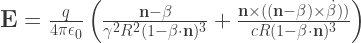
The magnetic field has a similarly involved expression, so rather than writing it out I’ll point you to the Wikipedia page.

In this expression, is the velocity of the particle divided by the speed of light, is the relativistic factor of the particle, is the distance from the particle to the observer and is the unit vector from the particle to the observer.

This is fairly complicated to look at, but there are a couple of interesting things we can pick out. The intensity of the radiation will scale like , so the first term will drop off like . The total area of a sphere receiving this radiation at only has area , so the total energy received goes like . This is then a non-radiative term – the particle is producing an electric field but this field isn’t propagating out to the observer. In fact, this term simply acts to move the field along with the particle.

The second term is more interesting, the intensity scales like , so the energy received by a sphere at radius is constant – this is just electromagnetic radiation. From the appearing we know it is nonzero only when the particle is accelerating.

We can integrate this expression over all observer angles and find the total power emitted by an electron travelling in a circle – this is the situation at CERN where charged particles travel in a giant ring of radius :

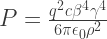
The killer for CERN is that factor – if you double the energy of a particle, it radiates 16 times more energy. In the case of electrons, this very quickly becomes such a high power that the accelerator can’t accelerate any more – the electrons radiate away their energy quicker than it can be pumped in. For protons of the same energy, their factor is times smaller, so radiate much less. This is why the LHC is so big, and uses protons rather than electrons. There are plans to build an even bigger LHC, unimaginatively called the Very Large Hadron Collider, or to accelerate electrons in a straight line so that they radiate much less energy at the proposed International Linear Collider. Both of these propositions are very expensive though, and very large, so there is much interest in smaller accelerators like plasma accelerators.

Anyway, that’s a lot of words and not much to look at, so how about some soothing animations? One thing which I glossed over above is the fact that these expressions for the electromagnetic fields need to be evaluated at the retarded time. In the words of my old undergraduate lecturer, lets do this in a retarded kind of way.

 

In one dimension, assume we are observing a particle at time and observer position . The particle emits radiation at the speed of light, so when we see radiation it has been emitted by the particle some time ago. We should take this into account when evaluating the appropriate electromagnetic fields, and evaluate at the retarded time. This is defined implicitly by the equation

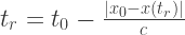
and encodes the fact that electromagnetic disturbances travel at the speed of light. In the general case this equation must be solved numerically if we want to use the Lienard-Wiechart potentials to make some pretty pictures. In effect we are travelling back from the observation point to the emission point along a lightcone. Once we intersect the particle path, we know the retarded time and the position/velocity/acceleration of the particle at the retarded time.

This sounds a bit tricky, but luckily for you I’ve had plenty of wet Saturday afternoons recently to do some simulations. First off, a particle going round in a circle with :

The top left represents the Poynting flux , or the radiation which would be observed. The retarded time is plotted beneath, and the two components of the electric field are plotted on the right. You can see how the retarded time is trailing the particle, and spreads out in a circle at the speed of light.

We can turn up the energy a bit, now :

Here the electron is much closer to the speed of light, and is consequently chasing it’s own lightcone – notice how there is a much larger jump in retarded time (from yellow to green). This causes the Poynting flux to be squeezed into a smaller time window, it’s much more compressed, intense, and energetic. The temporal shortening of the radiation pulse corresponds to a broad bandwidth, and it is precisely this pulse of radiation that corresponds to broadband synchrotron radiation.

What about something less extreme, an electron travelling at constant velocity in a straight line, again at :

We now see the action of the first term in the expression for the electric field – the field is being dragged along with the particle, but otherwise not radiating. Because the electron is travelling significantly slower than the speed of light, the field looks relatively undistorted. If you squint you’ll notice that the transverse field is stronger than the longitudinal field, which is a manifestation of special relativity (Lorentz transforming a uniform field back into the lab frame where the charge is moving).

Back to something more interesting, a simple dipole motion at :

We see what we hoped for, oscillating radiation perpendicular to the dipole, and zero far-field radiation parallel to the dipole. In the near-field (close to the dipole), there are electric field components everywhere, but it is clear that these must correspond to non-radiative terms and they die off rapidly.

Finally, let’s turn to a use for this radiation: undulators/wigglers. These are machines which purposefully oscillate an electron bunch to force synchrotron radiation emission, where the electron travels with high velocity in one direction and oscillates in the other:

You’ll see that unlike the dipole, the radiation field is asymmetric – the radiation in the direction of the electron has much higher frequency. In fact, the frequency is times the electron oscillation frequency (relativistic Doppler shift), which means for energetic electrons we quickly reach the hard x-ray range. This is great for imaging purposes, we can oscillate electrons and produce hard, collimated, bright x-ray beams. This is another area where plasma accelerators help to shrink down the required technology and beamline length.

Bumping up to a of 5, my animations now don’t resolve the radiation wavelength, and the high-energy radiation is compressed into a short pulse ahead of the electron.