Since Christmas, at my house we’ve been cooking with 5 ingredients or fewer thanks to the acquisition of Jamie Oliver’s new book, the contents of which are mostly available online here. The recipes are unanimously very tasty, but that’s besides the point. The real mark of culinary excellence (in my humble opinion) is how efficiently one can buy ingredients to make as many of the recipes as possible in one shopping trip. Let’s investigate while the lamb is on.

Each of the 135 recipes in the book consists of 5 ingredients, some of which overlap. It is therefore not necessary to purchase 675 ingredients, there are actually only 239 unique ones. (Yes, I did spend a Sunday morning typing 675 individual ingredients into a spreadsheet.)

The question is then this:

In which order should I buy my ingredients to maximise the number of possible recipes as a function of number of ingredients?

Let’s start simply, and look at the frequency of occurrence of the ingredients.

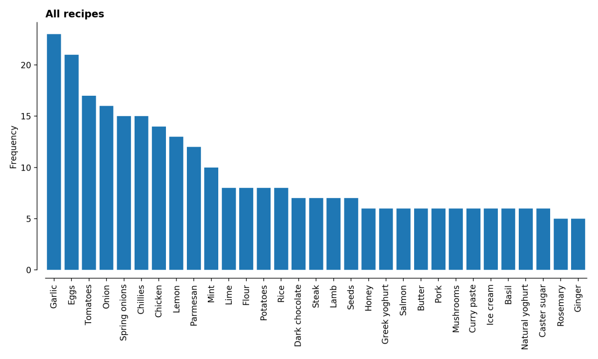
Unsurprisingly, the staples are prominent in these recipes – garlic, eggs, tomatoes, onions etc. are all things you might expect to find in a kitchen. At the other end of the scale are such mysteries as ras el hanout and pearl barley.

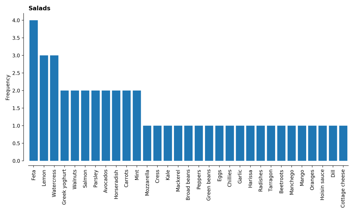
The book is helpfully categorised, so we can look for example at the distributions among, for example, salads and desserts, which all look sensible indeed.

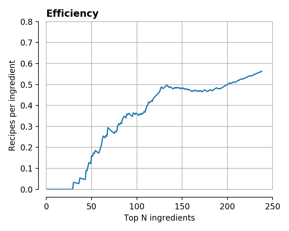
Let’s then think about how it is possible to define a successful ranking of ingredients. Clearly there is already one possible ranking – take the ingredients in order of their popularity, then count how many recipes it is possible to make with 5, 6, 7 … etc. of the ingredients.

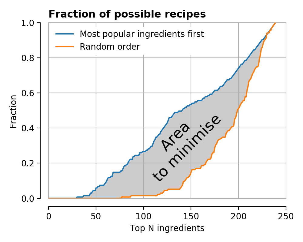
This fraction is plotted below, both as a ‘fraction of possible recipes’, and an ‘efficiency’ – the number of recipes per ingredient as a function of total number of ingredients.

At first sight this might look fine, but a closer look reveals that it is not a great ordering – it is impossible to make any recipes at all until you’ve purchased nearly 30 ingredients!

At second sight this fact is unsurprising, many recipes require at least a single ‘special’ ingredient which make the dish interesting beyond a mish-mash of the usual staples. The ‘popularity’ ordering here ignores this observation, making it decidedly sub-obtimal.

We can take this visualisation idea and plot different curves for different recipe orderings. In the following the orange curve represents the reverse-popularity ordering, where the least popular ingredients are chosen first.

Clearly this strategy is worse. Picking a totally random order of ingredients gives the green curve (and other random orderings the many grey curves), falling somewhere between the two extremes.

You can now start to see how it is possible to define a ranking for one recipe ordering with respect to another – find the area between the two cumulative distribution curves defined in this way.

The economically minded of you might note this is almost exactly the way a Gini coefficient is defined for relative equality.

What we will do then is take a random ordering, and adjust it such that it approaches and exceeds the curve defined by the ‘popularity’ ordering in blue. In this post I’ve taken the simplest and therefore probably slowest approach, which is to randomly permute two ingredients in the ingredient list, calculate a new ‘Gini’ curve, and see if the ‘fitness’ F has improved. If so, accept the permutation and try again 9,999 times.

Mathematically, what I’ve said above is

where ‘perm’ is a permutation of ingredients, G is the Gini curve, pop is the (static) curve of the popularity ordering, and N is the number of ingredients. We would like to pick the best ‘perm’ which maximises F. Unfortunately there are 239! = 1e66 possible orderings, so they can’t all be checked.

One final tweak to try and help the optimisation procedure is to add a weighting function, which can help by focussing attention on certain parts of the curve. Here I chose a couple of weighting functions, which rewarded improvements at the low-N parts of the curve more than the large-N parts, e.g. one example is a linear weighting

The idea here was to bump the orange curve up on the left-hand side, and make sure that it is possible to start making recipes with as few ingredients as possible.

OK, enough maths, let’s look at the results below. For several different weighting functions (the details are as it turns out unimportant), the Gini curves are plotted below.

It is very clear that we have improved on the naive ‘popularity’ method by a large amount in all cases, and actually most of the methods converged to very similar results. The big difference in the ‘offset’ case was that I was actively dissuading the high-N parts of the curve to try and focus attention elsewhere, but it seems to have made little difference.

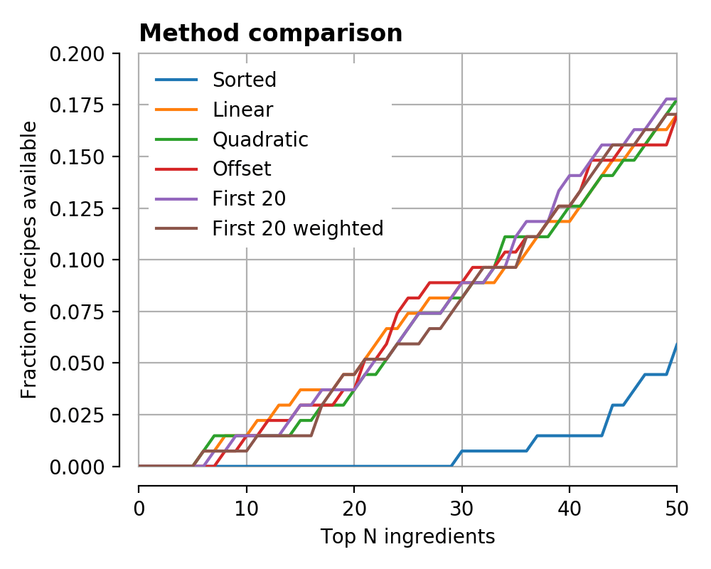
If we zoom in below, we see that in all of the new, more optimal, cases, it is possible to start making recipes nearly straight away. By the time the ‘popularity’ ranking has hit one recipe, we’re already on 12-14.

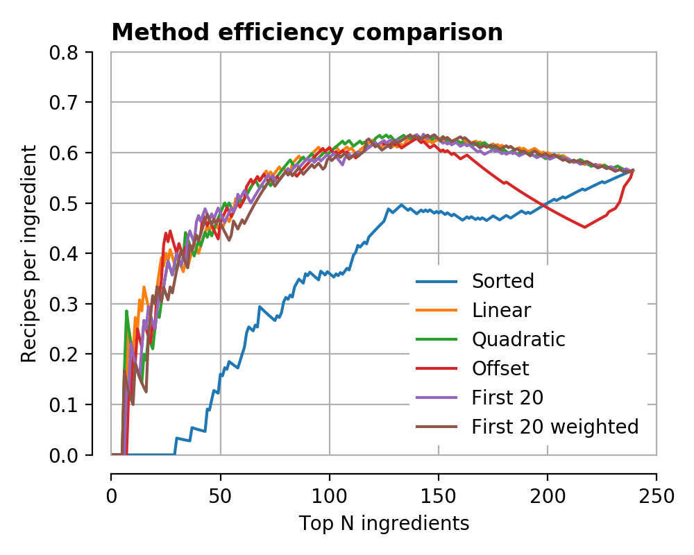
Looking at the ‘efficiencies’, the improvement is similarly apparent, reaching a peak efficiency somewhere around 150 ingredients.

This is great news, and worrying support for my terrible optimisation habits, but I’m sure the question you have is – what should I buy first?

Here the methods differed quite a bit, for example one prefers desserts with kimchee:

1. ‘Caster sugar’
2. ‘Eggs’
3. ‘Rice’
4. ‘Dark chocolate’
5. ‘Rye bread’
6. ‘Butter’
7. ‘Oranges’
8. ‘Kimchee’
9. ‘Chillies’
10. ‘Tomatoes’

And another enjoys Asian flavours with its citrus fruits.

1. ‘Hoisin sauce’
2. ‘Eggs’
3. ‘Seeds’
4. ‘Aubergines’
5. ‘Spring onions’
6. ‘Chillies’
7. ‘Chicken’
8. ‘Oranges’
9. ‘Lemon’
10. ‘Teriyaki sauce’

There’s no accounting for taste I suppose.

Code

The Jupyter notebook is available on Github, though I’ve not included any of the data as it came from a nice glossy book.