Swing and a miss

After my last post, where I noted that 45 degrees was the optimum angle to shoot a projectile the farthest, a commenter asked if the same was true for jumping from a swing. “Of course!” I initially thought. As we shall see, it isn’t actually that simple.

Setup

Let’s first, as usual, define the problem. Consider the following setup, where a swingee (one which shall soon be swung from a swing (say that three times fast (what are the grammatical rules for nesting parentheses?))) begins their swing at an angle $\lambda$ , and leaves the swing at an angle $\theta$ travelling at speed $v$ . The swing has height $h$ , though that doesn’t affect the result.

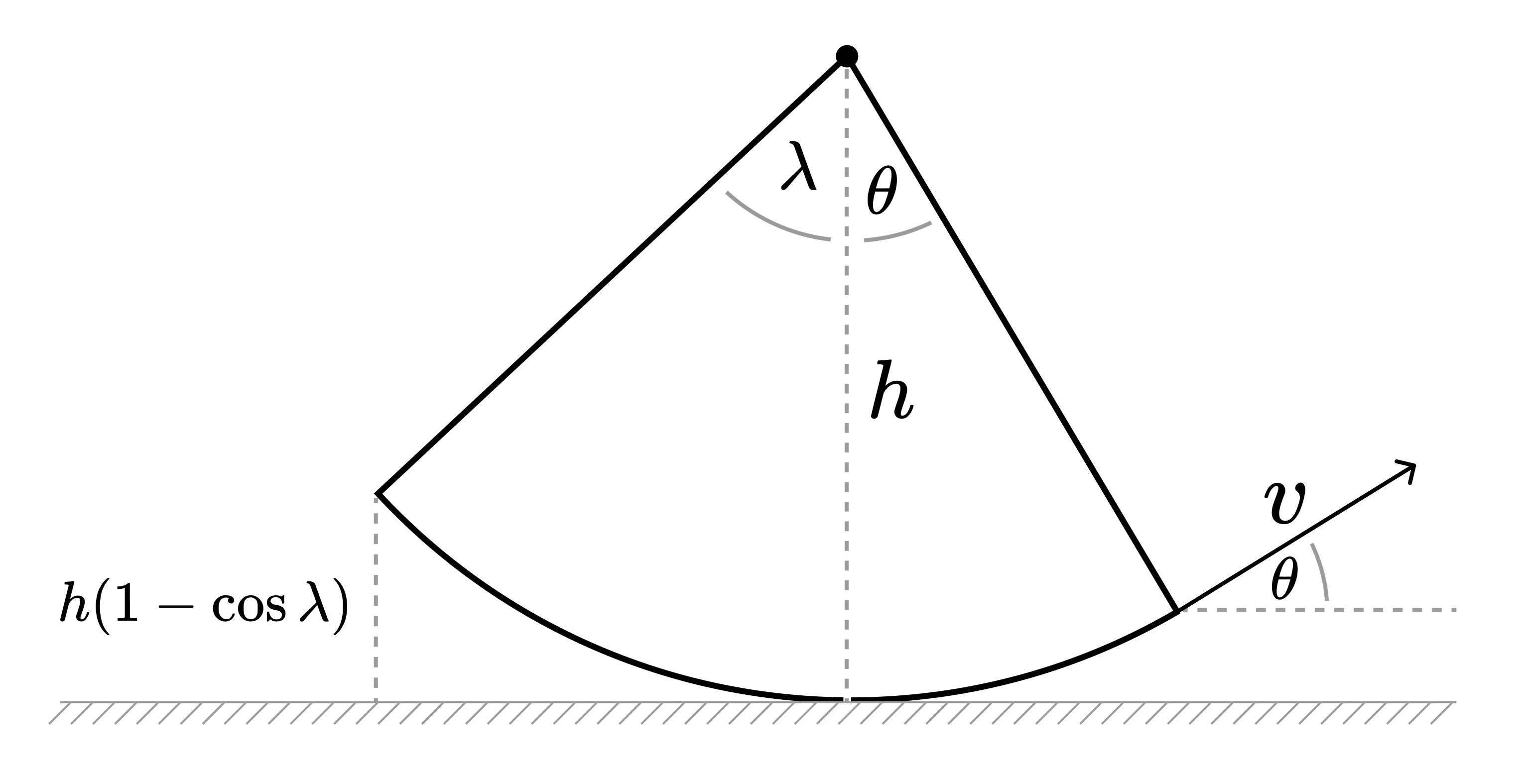
Let’s also assume that the swingee leaves the swing and then flies until they reach the ground (denoted by the hashed region above).

Following a similar approach to the last post, we immediately know that the equation of motion in the vertical direction is

$\displaystyle{y(t) = y_0 + v_0t - \frac{1}{2}gt^2}$

and that the initial conditions at $t = 0$ are

$\displaystyle{y(0) = h(1 - \cos\theta), \quad \dot{y}(0) = v\sin\theta}.$

In contrast to last time, here we also know the velocity $v$ . By conservation of energy we have

$\displaystyle{mg\Delta h = \frac{1}{2}mv^2 \Rightarrow v = \sqrt{2gh(\cos\lambda - \cos\theta)}}$

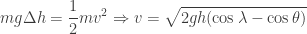
and so the equation of motion in the vertical direction becomes

$\displaystyle{y(t) = h(1 - \cos\theta) + t\cdot\sin\theta\sqrt{2gh(\cos\lambda - \cos\theta)} - \frac{1}{2}gt^2}.$

Solution

Trudging through some more algebra, the distance the swingee travels in the horizontal direction before landing turns out to be (deep breath)

$\displaystyle{\frac{x}{h} = \sin\theta\cos\theta(\cos\theta - \cos\lambda)\left(1 + \sqrt{1 + \frac{2}{(\cos\theta - \cos\lambda)(1 + \cos\theta)}}\right)}.$

This looks pretty imposing – let’s plot it as a function of $\theta$ and $\lambda$ to get some intuition about its behaviour.

The valid ranges of our variables are $0 < \lambda < \pi$ and $\theta < \lambda$ (by conservation of energy).

Here we’ve ‘solved’ the optimisation for $x$ numerically – for each maximum swing angle $\lambda$ , we find the approximate exit angle $\theta$ which maximises $x$ . These optimum angles are plotted in red on the left, and the maximum $x$ is plotted on the right. For an average $\lambda \sim \pi/2$ , you can expect to be launched a distance around 1.5 times the height of the swing.

Jump off the swing too early and you don’t go very far – your velocity is almost all horizontal, so you fall to the ground quickly. Jump off too late and your velocity is almost all vertical, wasting potential horizontal velocity. The best angle is, as expected, a function of your starting swing height ( $\lambda$ ).

For very small angles, your exit angle should apparently be about two-thirds of your maximum swing angle. For large angles, you should try and exit at around 45 degrees ( $\pi / 4$ ). This makes sense – as your exit speed $v$ gets larger and larger, the characteristic ‘gravitational length-scale’ $L_G = v^2/g$ gets large compared to the ‘swing length scale’ $L_s = h$ , and so any specifics of the swing situation stop mattering (such as the exact height of it), and you should be treated as a free particle.

The devil, as always, is in the details though, so let’s see how close we can get to an exact solution.

Analytical solution

The task now is to optimise the equation for $x$ with respect to $\theta$ , i.e. find the optimal $\theta^*(\lambda)$ that solves

$\displaystyle{\frac{\text{d}x}{\text{d}\theta} = 0}$

Just for fun (for a given value of ‘fun’), let’s write out this equation in full. Let $\vartheta = \cos\theta$ and $\ell = \cos\lambda$ , then we have to solve the following for $\vartheta$ :

$\displaystyle{\left(2\vartheta - \ell - \frac{\vartheta^2(\vartheta - \ell)}{1 - \vartheta^2}\right)\left(\sqrt{1 + \frac{2}{(\vartheta+1)(\vartheta - \ell)}} + 1 + \frac{2}{(\vartheta + 1)(\vartheta - \ell)}\right) - \frac{\vartheta}{\vartheta+1}\left(\frac{2\vartheta+1-\ell}{(\vartheta+1)(\vartheta-\ell)}\right) = 0}$

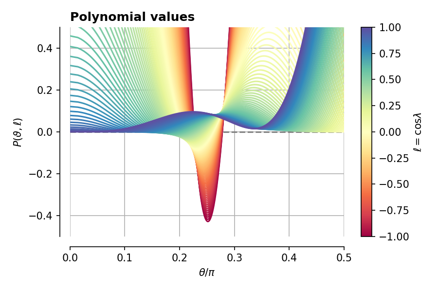
or in the form of a seventh-order polynomial in $\vartheta$ ,

$\begin{aligned}&\vartheta^7 \cdot 6 \\ +\,& \vartheta^6 \cdot (6 - 16\ell) \\ +\,& \vartheta^5 \cdot (14\ell^2 - 16\ell + 6) \\ +\,& \vartheta^4 \cdot (-4\ell^3. + 14\ell^2 + 2\ell - 12) \\ +\,& \vartheta^3 \cdot (-4\ell^3 - 12\ell^2 + 20\ell - 11) \\ +\,& \vartheta^2 \cdot (6\ell^3 - 11\ell^2 + 12\ell + 9) \\ +\,& \vartheta \cdot (2\ell^3 - 12\ell) \\ +\,& 4\ell^2 - 2\ell^3\\ =\,& 0\end{aligned}$

Sadly, there is no generic solution for seventh-order polynomials, but we can calculate their roots to the precision we desire. Doing this, and comparing to the rough solution above, we can at the very least see that our algebra was on-point.

Looking at the polynomial itself one can also see the various real roots. Who knows if they have any physical significance?

Here the red and yellow regions denote roots – places where the polynomial reaches values close to zero.

Thanks again to commenter Mike for prompting this post – as if I needed any further proof that I can be nerd-sniped at the slightest provocation.

One thought on “Swing and a miss”

mariusfrank says:

February 8, 2021 at 6:23 am

Mr Frank here (Marius to you now!). Great to see you still thinking! If I recall when you arrived in Year 7 we realised that normal input might not be enough and so I think we got in someone from the University to do some coaching. Is that right? I can’t remember. Clearly there has been some impact! Love to hear from you about what you’re doing. I stay in touch with Vicky via FB. Take care Marius (Mr Frank)

LikeLike

Almost looks like work

Swing and a miss

One thought on “Swing and a miss”

Leave a Reply Cancel reply

Share this:

Like this:

Related

One thought on “Swing and a miss”

Leave a Reply Cancel reply