When initially fiddling around and getting to grips with Matlab a while ago, I had a go at implementing the ‘logistic map’, a well known mathematical process which leads to deterministic chaos.

http://en.wikipedia.org/wiki/Logistic_map

The mathematical operations involved are extremely simple, namely for some value of we repeatedly perform the operation

.

Starting at , after a single iteration we should end up at , and after another we should be at . Continuing this process, you might expect that we should converge on some function which stipulates . Calculating this function is trivial, we look for a ‘fixed point’ of the map above and solve:

.

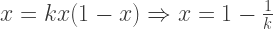If we plot a few iterations and our ‘solution’ below, note a few interesting things.

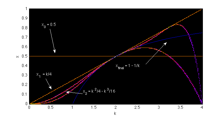
The functions are all bounded between 0 and 1 for , and increase in polynomial order as we increase the number of iterations, much like a Taylor series. However, the ‘final’ function contains a term , which can’t be approximated by a finite number of positively-powered polynomial terms. In other words, no matter how many iterations we produce, our resulting functions will never contain a term and so will never quite reach the ‘actual’ function.

This reminds me slightly of a calculation in condensed matter field theory, where the pairing potential between electrons is calculated to be of the form , where is some (assumed small) interaction between electrons. This is then a non-perturbative result, as no amount of perturbation orders, i.e. terms proportional to , will lead to a function containing a term.

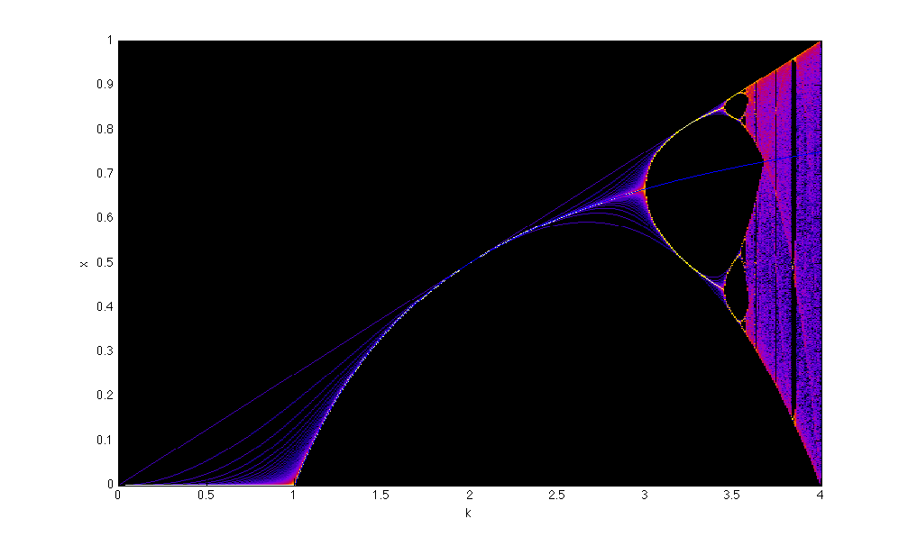
Anyway, physics distractions aside, we can continue this iteration process and see where we end up.

All of the iterations up to 1000 are plotted on top of one another, the first one is visible, and successive iterations converge upon the blue line representing . Great! That is, until where something funky happens – the line splits into 2 and diverges from our supposed solution.

Like all great experimental scientists, we should examine our theory again in light of new evidence. Guided by what we’ve seen, lets suppose there exist 2 solutions to our map, call them and . Then we have

.

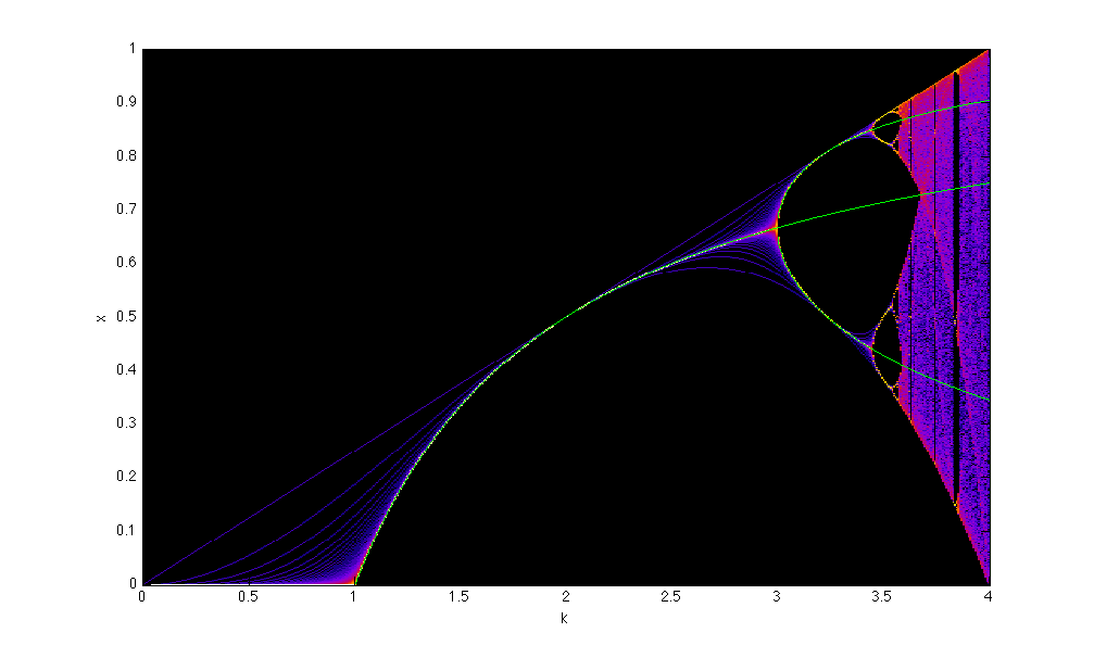
This is a cubic equation with 3 solutions (thank you symbolic algebra toolbox!):

Accounting for the possibility , one of the solutions ends up being our original solution which is nice. The second two represent the two new branches of the map above , and as we can see plotted below, fit very nicely. Also, we see why the branches occur at this point – the new solutions become imaginary for and so the map reverts back to the single solution again.

Unfortunately, at around the map splits again, and in solving for this we would have to deal with a 15th degree polynomial, which isn’t ideal. However, by dividing out the above solutions (because 1 and 2 are factors of 4, then the above solutions must be included as we could have all 4 solutions the same, or two sets of two) we end up with a 12th degree polynomial, and by investigating its discriminant we find the onset of the 4 solutions at .

This doubling process occurs quicker and quicker until in a finite period we end up with chaos – the mess above . Nevertheless there are still patterns in here, hinting at the underlying deterministic order. We can zoom in and we find smaller copies of the overall pattern

and so again in this blog we have what looks like a fractal. Nothing as fancy as complex numbers need get involved here, just the kind of equation you could understand in secondary school, and eminently simple to visualise if you feel like a bit of programming on a wet Sunday afternoon.