What do black holes look like?

From a recent post I’ve had the scripts lying around to calculate the trajectories of particles around black holes. The paths were pretty crazy, which got me wondering what such a system would look like. For that I need to calculate how photons move around black holes, which is a slightly different problem, and doesn’t offer up much in the way of puns for post titles…

Black holes of course don’t emit any light, and don’t reflect any light. These are the two mechanisms by which we see most objects, which won’t work for a black hole. Instead we’ll have to consider how the gravitational field of the black hole distorts the path of light travelling nearby. For the sake of simplicity, we’ll only consider one black hole which distorts the image of a scene far off into the background.

To think about how to approach this problem, consider the fancy 3D drawing below. Without the black hole present, an image is formed on a camera when light rays from the background scene hit the lens. This background is emitting light in all directions, so the most efficient way of calculating what the image looks like is to go backwards – send light rays out of the camera and see where they end up on the background. Do this for each pixel in the camera and you end up with an image. As the object is ‘infinitely far away’, different pixels just correspond to different light ray angles.

The presence of the black hole distorts these light rays – in the example above a ray which might normally sample a part of the background way out to the top will actually sample a region near the middle. Other rays will end up inside the black hole, and so the corresponding pixel will be black. The task is then, for every pixel in the camera sensor, calculate the trajectory of a photon leaving the camera and passing round the black hole and see where it ends up. For a decent image this might require $10^6$ rays, which is a lot of computational effort. Instead we can do something simpler – due to the symmetry of the problem we just need a map of angles ‘in’ to angles ‘out’ – plotted below.

We send a ray out of the camera at angle $\theta_{in}$ , calculate its path (blue) to a point where it’s travelling in mostly a straight line, and measure the new angle $\theta_{out}$ . Do this for enough $\theta_{in}$ s and we can find the function relating input and output angles $\theta_{out} = f(\theta_{in})$ . This function is then easily applied to transform the background image in a single step, and is much quicker than calculating the path for each pixel. I will neglect gravitational redshift in this approximation.

With a procedure outlined then, onto the first step: calculating photon trajectories. A point mass induces a Schwarzchild metric $g_{\alpha\beta}$ on its local spacetime, where the metric defines the length of ‘straight lines’ over coordinates $x^{\alpha}$ : $g_{\alpha\beta}x^{\alpha}x^{\beta}$ (assume Einstein summation convention).

The equations of motion are then

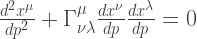
$\frac{d^2x^{\mu}}{dp^2} + \Gamma^{\mu}_{\nu\lambda}\frac{dx^{\nu}}{dp}\frac{dx^{\lambda}}{dp} = 0$

where the affine connection $\Gamma$ is related to the metric $g$ by

$\Gamma_{\mu\lambda}^{\sigma} = \frac{1}{2}g^{\sigma\nu}\left(\frac{\partial g_{\mu\nu}}{\partial x^{\lambda}} +\frac{\partial g_{\lambda\nu}}{\partial x^{\mu}} - \frac{\partial g_{\mu\lambda}}{\partial x^{\nu}}\right)$ .

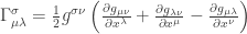
The parameter $p$ simply measures position along the trajectory. For massive particles this is most naturally the proper time of the particle, but for photons (where proper time doesn’t elapse) such an interpretation isn’t possible.

Crunching through the algebra then, the relevant equations of motion are

$\left(\frac{dr}{dp}\right)^2 + \frac{J^2}{r^2}\left(1 - \frac{2GM}{rc^2}\right) - c^4 = 0$

$r^2\frac{d\phi}{dp} = J$

where $(r,\phi)$ is the position of the photon as indicated in the diagram above, $M$ is the mass of the black hole and $G$ is the gravitational constant. $J$ is a constant of motion, identified with the angular momentum of the photon. Making the substitution $u = 1/r$ and tidying up a bit, the surprisingly simple result is the 2nd order ODE

$\frac{\partial^2u}{\partial\phi^2} + u = \frac{3GMu^2}{c^2}$

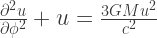
where we’ve eliminated $p$ such that we’re only interested in the shape of the trajectory. The initial conditions we need to supply are $u_0 = 1/r_0$ , $\phi = 0$ and $\left.\frac{du}{d\phi}\right|_0 = 1/(r_0\tan\theta{in})$ , which can be derived from a bit of geometry. For simplicity I’ll use units where $G = c = 1$ .

Plotted below are a few results for $r_0 = 20$ , and $0 < \theta_{in} < 60^{\circ}$ . The behaviour of the photons is dictated by their distance of closest approach. Too close and the photons spiral into the black hole, plotted red. A bit farther and the photons swing round the black hole severely. If you were to look in this direction then you’d be able to see round corners, or even see yourself staring back. Farther still and the photon paths become curved, but not excessively.

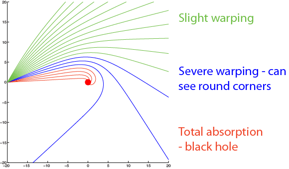
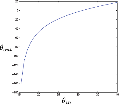
The relation between input and output angle is plotted below, and reflects what we see above. For large $\theta_{in}$ the deviation is small, around $20^{\circ}$ . At some point $\theta_{out}$ drops below zero, which is when we start seeing round corners, and below $15^{\circ}$ the photons are just absorbed.

What does this look like? Well I can apply the above function to an image to produce the following, assuming a field of view of about $60^{\circ}$ . The black hole is a bit farther away in order to make the image clearer.

Pretty nice! From the above we can see that some photons get bent right back around, for which I need a ‘background’ image in all directions. For simplicity I just tiled the background, which is why right in the middle, where the ‘blue’ rays might be going, you can see a few different bright spots corresponding to the bright patch on the left.

That isn’t to say that multiple images don’t occur, as the second image of the bright cloud on the right hand side of the black hole is indeed a gravitationally-induced second image. The light has bent around the back of the black hole and is shot towards the camera.

The obvious ring that you can see is an Einstein ring. This is a position where $\theta_{out} = 0$ , satisfied for a ring of points around the camera. A single object in the background is then mapped to a ring in the image, and these have quite amazingly been observed in astronomy, see the linked Wikipedia page for a lovely example.

Everything is better when animated though, so scrolling the background a bit we get this

Or in a higher-quality Youtube version here:

Of course we don’t just have to use space scenes, what if one really did appear at the LHC?

It probably wouldn’t do the beam pipes much good…

There are a few more things which would be interesting to explore with this procedure. For example, using high-quality environment maps to get a proper 360-degree view rather than tiling the same image. Also, for small angles, the light rays wrap around the black hole an increasing number of times. This gives rise to multiple Einstein rings at closer and closer intervals. I could also make an animation of what the approach to a black hole looks like. All fun things to do, but they’ll have to wait until next time as my typing fingers are starting to give out.

11 thoughts on “What do black holes look like?”

It might be neat/useful to put something more easily identifiable as the background. You could put several uniquely colored dots or shapes around on the background so we could watch how it gets distorted. If I knew that a green circle was behind me, red in front, blue to my left, and yellow to my right, I would be able to much more easily see how the blackhole warps things and how the Einstein ring works.

LikeLike

Might be cool to have a different background so we could see how the warping happens more easily. Not sure how you’ve done the space (if it’s the inside of a sphere or a box or whatever), but you could put uniquely-colored shapes every 90 deg (on each wall, so to speak). That way, when you rotate around the blackhole, you can clearly see how everything gets warped.

LikeLike

jasmcole says:

October 11, 2014 at 8:27 am

Yes that’s a good idea. My warping method just spits out a radial direction in spherical coordinates for every image pixel, so a procedurally-generated background would be easy enough to implement.

LikeLike

Reply

Pingback: What It Would Be Like To Fall Into A Black Hole | Sharing Interesting Stuff, Updates News & Free Tips

What did you use to “apply the above function to an image”? I want to replicate the same thing on my part but am not sure how to use the angle function to manipulate the image.

Thanks!

LikeLike

jasmcole says:

January 24, 2015 at 11:27 am

Hi, for this I actually work backwards. I have a precomputed lookup table linking thetain and thetaout. In the output image I scan through pixel by pixel, and for each one calculate thetaout, which just depends on the field of view of the camera. I then look up which value of thetain this corresponds to and grab the correct pixel colour from the background image.

LikeLiked by 1 person

Reply
1. Aashish Tripathee says:
  
  January 25, 2015 at 6:10 am
  
  Hi,
  Thank you so much for the reply.
  
  How did you calculate theta_out = f(theta_in)? I tried using some geometry there but I cannot see any restriction on theta_out that the other parameters impose. I do have the relation between r and phi but I’m not sure how that’s relevant to theta_out though the amount of bending of the ray would be dictated by the geodesic equation which ultimately is hidden inside the relation between r and phi.
  
  Thanks a lot and sorry for bothering you!
  
  LikeLike
2. jasmcole says:
  
  January 25, 2015 at 10:57 am
  
  Hi, I initialise a ray at the camera plane at some value of theta_in. I then step through the ODE to find the ray path around the black hole, and when it reaches a sufficient distance stop and calculate the new propagation angle – theta_out. I don’t know if there’s an analytical solution for the ray path though, there will be for small deflections, but probably not for these large ones.
  
  LikeLiked by 1 person
3. Aashish Tripathee says:
  
  January 26, 2015 at 6:48 am
  
  That makes so much sense now. Thanks a lot!
  
  LikeLike

Hello,

I have been reading the blog moths ago and this post really impressed me!

Sorry for the bothering. I’m also trying to replicate the work for a my final essay for my physics career and i have some questions if you don’t mind. It would be great to have some advice from you.

I don’t get how you can assign theta_in to the camera grid (when you form the image). I mean, the problem is in 3D (I know that as the solution lies in a plane, is angular-invariant) and therefore you need at least two coordinates in the grid. For example, theta_in and phi…..which i suppose that would be drivated from the x-y position of the grid using spherical coordinate transformations (having the distance of the observer to the grid). Maybe i’m making this more problematic that already is….but i really don’t get the algorith to assign the theta_in to the grid (that i suppose is discretized).

Also, the equation for u has a solutions that reach u=0, what means r=inf for diferent values of phi deppending of the initial value of theta_in. What is your criteria to get the adecuate phi to calculate theta_out?

And finally (and really i beg pardon for this) i’m unable to relate u'(0) with theta_in geometrically. If you can point some directions to get the relation that you provide….it would be great. (I know, shame on me).

Thanks you for all and i really apologize for the bothering.

Kind regards!

(And sorry for my bad english)

LikeLike

jasmcole says:

January 29, 2015 at 10:56 am

Hi, glad you like the post (and your English is great!). The key to assigning directions to camera pixels is that we are assuming the background is ‘at infinity’, and the camera lens is exactly the focal length from the CCD. In this case, only the direction of the light rays hitting the lens matter, and for a perfect lens different directions are just mapped to pixels – this is why I only consider the angle of light rays, not their positions.

You are correct though, we need another angle on the camera plane going around the centre, which we can call A. What I do is loop through the camera pixels, work out which theta_out they correspond to (which only depends on the radial coordinate of the pixel), and match that to a theta_in. Now the A coordinate is unchanged when going around the black hole due to symmetry (this wouldn’t be the case for e.g. a Kerr black hole), so I use the A coordinate from the camera plane to look up the background pixel coordinate.

In summary (x,y)_camera -> (theta_out,A)_camera -> (theta_in,A)_background -> (x,y)_background

I may have confused you a bit with my variable names, (theta,phi) don’t form a spherical coordinate system. Theta is just the angle a ray makes with the optical axis, phi is an internal variable I use when computing the light ray paths.

I terminate the ODE when u gets small enough (when r gets very large), and then calculate the slope of the ray to get theta_out. An easy way to check that you’ve gone ‘far enough’ is that actually in this ODE u can go negative and oscillate quite happily. This is obviously unphysical, so I just check when u is about to go negative and calculate the slope there.

Finally, if the ray starts at a radius r0 from the black hole, the initial slope is dudphi0 = 1/(r0*tan(theta_in)), which you can convince yourself of with a little bit of geometry.

Hope this helps!

Jason

LikeLike

Reply

Almost looks like work

What do black holes look like?

11 thoughts on “What do black holes look like?”

Leave a Reply Cancel reply

Share this:

Like this:

Related

11 thoughts on “What do black holes look like?”

Leave a Reply Cancel reply