A probability puzzle

I saw a ‘simple’ puzzle on the internet which I thought I’d have a crack at in an evening. Several furious scribblings on the bus and the sofa later, I finally have an answer. I’m so relieved I can’t help but share the joy.

The puzzle

Uniformly draw a random real number $r$ between $0$ and $N$ . Repeat, drawing a number between $0$ and $r$ . You lose the game when you draw a number below $1$ . On average, how many turns do you last in the game?

I encourage you to have a go at this problem, and please let me know if you find a simple way to the answer. I’ll describe my method below. I didn’t know the answer beforehand, so likely didn’t take the most direct route to it.

The first turn

We draw the number with uniform probability, so the odds of picking a number in turn 1 $r_1$ between $r_1$ and $r_1 + \delta r_1$ is just

$P(r_1)\delta r_1 = \frac{1}{N}\delta r_1$

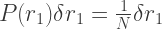
Simple. For illustration of this trivial example, I’ve plotted below the analytic solution for the probability density $P(r_1)$ and a histogram of some numerical samples from a uniform distribution.

It’s obvious what the chance of losing in the first turn is, but I’ll be explicit to clarify the procedure. We need to integrate $P(r_1)$ between $0$ and $1$ , or

$P(\text{lose}_1) = \int_0^1 P(r_1)\,\text{d}r_1 = \int_0^1 \frac{1}{N}\,\text{d}r_1 = \frac{1}{N}$

One turn down, $\infty-1$ turns to go.

The second turn

Here it gets a little trickier. There is some chance that we lost the game in the first turn, so if we integrate the probability of picking a number $r_2$ in the second turn we should get a number less than unity.

Carrying on regardless, by the law of total probability and the fact that the values of $r_2$ we can pick are dependent on the previous $r_1$ that we picked,

$P(r_2) = \int P(r_2 | r_1) P(r_1)\,\text{d}r_1$

The integration limits are very important here. The largest value that $r_1$ could take is $N$ . The smallest is $r_2$ , as remember we are picking a value such that $0 < r_2 < r_1$ .

From the first turn, $P(r_1) = 1/N$ , and similarly $P(r_2|r_1) = 1/r_1$ , so performing the integral

$P(r_2) = \frac{\ln(N/r_2)}{N}$

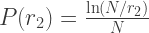
If we’ve made it to the second turn, it must have been that $r_1 > 1$ , and so the equation above is only valid for $r_2 > 1$ , as those values only receive contributions from the possibilities $r_1 > 1$ . There is obviously a chance that we can pick $r_2 < 1$ , but again these have only received contributions from the values $r_1 > 1$ . As $P(r_2)$ passes down through $r_2 = 1$ , the probability can’t increase, and so stays constant from $r_2 = 1$ to $r_2 = 0$ .

This two-part distribution is plotted below, and as you can see agrees with some numerical tests.

Here $N = 100$ , so the curve flattens at $r_2 = 1/100$ .

Here $N = 100$ , so the curve flattens at $r_2 = 1/100$ .

Also, integrating $P(r_2)$ ,

$\int_0^N P(r_2)\,\text{d}r_2 = 1 - \frac{1}{N}$

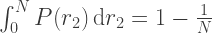
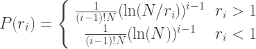
less than one as predicted, by an amount equal to the probability of losing in the first turn $P(\text{lose}_1)$ . The fact that it’s possible to lose the game is already priced in to these distributions, which will come in handy later.

The next turns

Armed with some insight on how to proceed, the distribution for the third turn is

$P(r_3) = \int_{r_3}^N \frac{1}{r_2} P(r_2) \,\text{d}r_2 =\int_{r_3}^N \frac{1}{r_2}\frac{\ln(N/r_2)}{N}\,\text{d}r_2$

This looks a bit nasty, but has a surprisingly pleasant solution

$P(r_3) = \left\{ \begin{array}{cc} \frac{1}{2N}(\ln(N/r_3))^2 & r_3 > 1 \\\frac{1}{2N}(\ln(N))^2 & r_3 < 1\end{array} \right.$

There’s looking to be a bit of a pattern here. Integrating $(1/x) \ln(N/x)^i$ by parts it’s possible to show the general solution for any turn (including the first one!)

$P(r_i) = \left\{ \begin{array}{cc} \frac{1}{(i-1)!N}(\ln(N/r_i))^{i-1} & r_i > 1 \\\frac{1}{(i-1)!N}(\ln(N))^{i-1} & r_i < 1\end{array} \right.$

Comparing this expression to numerical experiments, the agreement is very good:

The curves for each turn have been displaced vertically for clarity.

Winning and losing

Armed with this expression, the original question can be answered. First of all, what’s the probability of winning turn $i$ ? Integrating the above from $1$ to $N$ ,

$P(\text{win}_i) = 1 - \frac{1}{N}\Sigma_{n = 1}^{i}\frac{1}{(n-1)!}(\ln(N))^{n-1}$

You will recognise the right-hand side as the first $i$ terms of the Taylor expansion of $\exp(x)$ , so

$\lim_{i \rightarrow \infty} P(\text{win}_i) = 1 - \frac{1}{N}\exp(\ln(N)) = 0$

and as expected the chances of passing a turn go to zero for large turn numbers.

The expression for losing on turn $i$ is simpler, just

$P(\text{lose}_i) = \frac{1}{(i-1)!N}(\ln(N))^{i-1}$

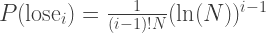
The cumulative probability of losing on turn 1, or turn 2, or … turn $i$ is the same sum as above, approaching $\exp(\ln(N))/N=1$ – everyone loses eventually!

When do I expect to lose

Getting back to the main point, when are these games lost on average? Plotting $P(\text{lose}_i)$ for a range of $N$ below, the number of turns goes up very slowly with $N$ .

It’s unlikely to lose too early, but also unlikely to lose too late. The distribution, as with all things, starts to look quite gaussian for large $i$ (exercise for the reader: show this by expanding $\ln (P(\text{lose}_i))$ about its maximum).

The expected turn to lose on is simply the sum over $i \times P(\text{lose}_i)$ . There is no normalising constant as we showed above that $\Sigma_i^{\infty} P(\text{lose}_i) = 1$ .

Performing this sum,

$\begin{array}{rl} E(\text{losing turn}) & = 1\times\frac{1}{N} + 2\times\frac{1}{N}\ln(N) + 3\times\frac{1}{N}\frac{1}{2!}(\ln(N))^2 + \dots \\ & = \frac{1}{N}\left(1 + 2\ln(N) + \frac{3}{2!}(\ln(N))^2 + \frac{4}{3!}(\ln(N))^3 +\dots\right)\\ & = \frac{1}{N}\frac{\text{d}}{\text{d}\ln(N)}\left( \ln(N) + (\ln(N))^2 + \frac{1}{2!}(\ln(N))^3 + \right)\\ & = \frac{1}{N}\frac{\text{d}}{\text{d}\ln(N)}\left( \ln(N) (1 + \ln(N) + \frac{1}{2!}(\ln(N))^2 + \dots)\right)\\ & = \frac{1}{N}\frac{\text{d}}{\text{d}\ln(N)}\left( \ln(N)\exp(\ln(N))\right) \\ & = 1 + \ln(N) \end{array}$

What a lovely result! Here it is plotted against some numerical tests.

nturns — As an experimental scientist, I’ve never seen such strong correlation 😦

One might have immediately suspected that logarithms were involved, given that the game involves repeatedly shrinking a number by some proportion. In fact, if there was no losing involved you can show that the expected number drawn on each turn is $N/2^i$ , i.e. on average the numbers halve each turn. The tricky part is incorporating the probability of losses, which manifests here as a trimming of the probability distributions below $r_1 = 1$ .

Exercises

Repeat for a loss at an arbitrary number $n$ rather than 1.

Repeat for the discrete case where $N$ and $r_i$ are integers.

Compute the limiting distribution of probability of loss over turns for large $N$ .

One thought on “A probability puzzle”

asving says:

October 1, 2016 at 6:28 pm

You can set up the problem as an integral /differential equation :

Let f(x) be the expected number of turns beginning with N=x. Then this function satisfies a recurrence relation.

f(x) = 1/x + 1/x integral_1^x (f(y) +1)dy.

The first term is what what happens when you roll less than 1 on your first turn, the remaining is the expectation for everything else. Isolate the integral and differentiate to get a simple differential equation.

Fun problem.

LikeLike

Almost looks like work

A probability puzzle

One thought on “A probability puzzle”

Leave a Reply Cancel reply

Share this:

Like this:

Related

One thought on “A probability puzzle”

Leave a Reply Cancel reply