Stochastic geometry and the London underground

Way back when I was analysing London house price data for the Summer Data Challenge, I made a histogram of the distances from a random point in London to the nearest tube station. I noted that it peaked around half a kilometre, but ignored the shape of the distribution itself. This is an unfortunate faux pas for the accomplished procrastinator, so let’s right that wrong with the help of some stochastic geometry.

The study of random spatial patterns is called stochastic geometry, and here we are most interested in a subfield which involves so-called point processes. This is the analysis of random distributions of points, as might be approximated by tube stations or, in the literature, mobile phone base stations.

Poisson point processes

A Poisson point process is one where the underlying distribution of points is Poisson. Given a mean density of points $\rho$ , the number of points $n$ lying within a given area $A$ follows the distribution

$P_P(n) = \frac{(\rho A)^n}{n!}e^{-\rho A}$

To simulate this, I take a unit square, split it into 400 small cells, and fill each cell with a random number of points which follow a Poisson distribution. The points are plotted below on the left. On the right I have sampled this distribution 100,000 times, measuring the number of points within a radius of 0.02 from a random point within the square. The agreement is good, suggesting that this is a good approximation to a Poisson point process.

PoissonPoints — Left: Poisson point distribution. Right: Measured and theoretical distribution of points within a radius of 0.02.

The only problem with this method is that the total number of points $N$ isn’t determined. Over many realisations $N$ will average to $\rho$ (given the unit area of the box), but there will be some variance.

Binomial point processes

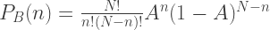
In real life there will often be a fixed number of points to consider, so it would be nice to incorporate this fact. The solution is to switch to a binomial point process, where a fixed number $N$ of points are scattered randomly within the square. The reason for the name comes from the probability distribution that this process generates. If we consider an area $A$ of the square, then the odds of a randomly chosen point lying within this area is $A/\text{area of square} = A/1 = A$ . The odds of finding $n$ points within this area is akin to getting $n$ heads out of $N$ coin flips when the coin is weighted such that the probability of a head is $A$ .

This is the standard binomial distribution, and so the number of points within an area $A$ is binomially distributed as

$P_B(n) = \frac{N!}{n!(N - n)!}A^n(1-A)^{N-n}$

It’s simpler to generate a binomial point process as one just needs a list of N uniformly distributed x and y co-ordinates, and as plotted below the agreement with the expression above is again good.

BinomialPoints — Left: Binomial point distribution. Right: Measured and theoretical distribution of points within a radius of 0.2.

Nearest points

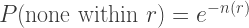
This is all good so far, and we can generate the distributions we need. However the original problem was to investigate the distribution of the distances to the nearest point in an array of points. To work this out we need the probability that there is at least one point within a distance $r$ :

$P(\text{at least one within } r) = 1 - P(\text{none within } r)$

For the two cases above we have (for the unit square case where $\rho = N$ )

$P_P(\text{at least one within } r)) = 1 - e^{-N\pi r^2}$

$P_B(\text{at least one within } r)) = 1 - (1 - \pi r^2)^N$

Finally, note that the probabilities here have been considered in a cumulative sense – we are calculating quantities within a certain radius. To get the probability density that the nearest point is actually at a certain radius requires the differentiation of the above

$P_P(\text{nearest station at } r) = 2\pi Nre^{-N\pi r^2}$

$P_B(\text{nearest station at } r) = 2\pi Nr(1 - \pi r^2)^{N-1}$

The astute amongst you will have noticed that for large $N$ these two expressions become very similar. For large $N$

$\lim_{N \rightarrow \infty} (1 - \pi r^2)^{N-1} = (1 - (N\pi r^2)/N)^N = e^{-N\pi r^2}$

This is because the fractional variations in $N$ for the Poisson process scale as $1/\sqrt{N}$ and so for large $N$ the total number of points is essentially fixed, matching the definition of the binomial process.

Here are histograms of the distance to the nearest point for a Poisson point process:

PoissonPointsNearest — The histogram of the distance to the nearest Poisson-distributed point to 1,000 randomly-chosen locations.

and a binomial point process:

BinomialPointsNearest — The histogram of the distance to the nearest binomially-distributed point to 10,000 randomly-chosen locations

In both cases the match is good, and so my maths isn’t completely terrible.

Fitting to the data

This is good, we understand how to model the distance to the nearest point in a couple of random distributions. How does this match up to the London tube station data?

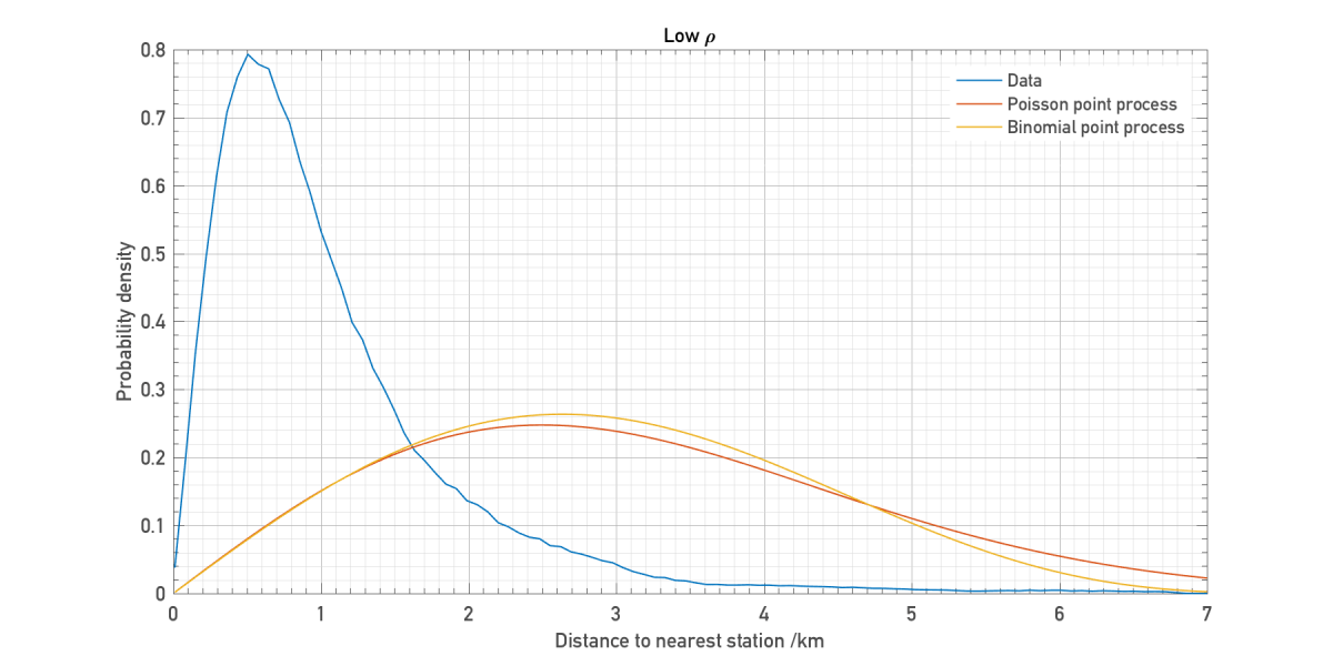
Let’s see how the distributions above compare for low density:

DataFitLo — There are slight differences between the models in the low density case…

And high density:

… and in the high density case the models rapidly converge.

It seems that we cannot reproduce the actual distribution with a simple model like this. In particular there is a long tail which is never matched by either the Poisson or binomial model. At the high densities required to get the peak in the right place, it becomes very unlikely that the nearest station can ever be very far away.

The key here is that London’s tube network isn’t homogenous like these point processes. It has a high density core surrounded by a low density halo, and so the model should be tweaked to account for this.

Let’s suppose that the station density varies as a function of distance. The number of stations within a radius $r$ is now

$n(r) = 2\pi\int_0^r r'\rho(r')\text{d}\,r'$

And so the Poisson point process is modified such that

$P(\text{none within } r) = e^{-n(r)}$

Churning through the same algebra as above, we get that the distance to the nearest station follows the distribution

$P_{nearest}(r) = 2\pi r\rho(r)e^{-2\pi\int_o^r r'\rho(r')\text{d}\,r'}$

Now we have measured $P_{nearest}(r)$ , so the challenge is to find a $\rho(r)$ which satisfies the above constraint. It is possible to write down a differential equation which $\rho(r)$ satisfies, but I found that numerical solutions of this equation became very noisy and behaved unpredictably. Instead, I took a very simple approach and randomly tweaked values of $\rho(r)$ one at a time. If the match with the data was better, following the above transformation, accept the tweak and move onto the next one. In this way I converged to a solution. I also added a term penalising large derivatives in $\rho$ to avoid spurious oscillations.

As plotted below the fit works well, matching the long tail of the actual distribution.

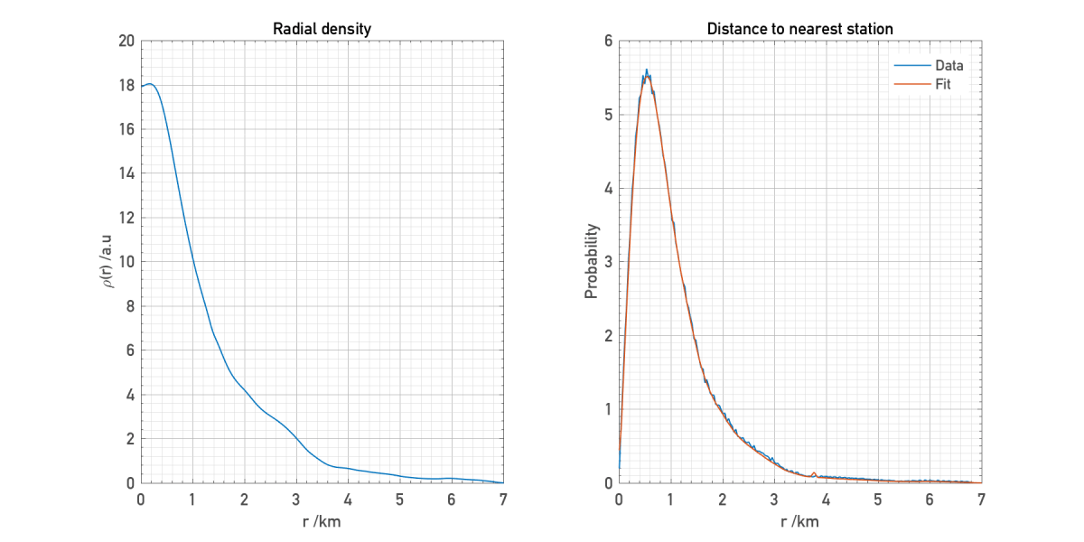
Fitted radial distribution of station density.

Though expected, it’s nice to see that the retrieved density matches the description outlined above. A dense core which quickly drops off after a few kilometres. Note that this is the average distribution as witnessed by many random observers plonked somewhere within London, so doesn’t correspond to the actual radial distribution of stations. However I find the fact that, in principle, it’s possible to calculate something like this from a simple observation of the distance to the nearest station pretty cool.

Code

You can access the scripts I used to make the plots in this post at the Github repository for my blog here.

Almost looks like work

Stochastic geometry and the London underground

Poisson point processes

Binomial point processes

Nearest points

Fitting to the data

Code

Further reading

Leave a Reply Cancel reply

Poisson point processes

Binomial point processes

Nearest points

Fitting to the data

Code

Further reading

Share this:

Like this:

Related

Leave a Reply Cancel reply