Newton’s 4th Law

This post is about me finally getting over a slight irritation that happened nearly a decade ago, one which was almost completely inconsequential. Fortunately, it was related to physics, so is fair game here.

Back during my undergraduate days, part of the teaching process came in the form of supervisions, whereby an academic would lead a discussion with one or two students and grill them on their weeks work. One time, I confidently answered a question about heat transport by quoting something I remembered called ‘Newton’s law of cooling’, describing how temperature differences changed with time. My supervisor told me that there was no such thing, and elevating such a concept to a ‘law’ was far too grandiose. I meekly accepted their condemnation, and we swiftly moved on.

I’ve finally recovered from this episode, so let’s take a more thorough look at what Newton was on about.

Newton’s law

Now Newton’s law of cooling is definitely a real thing, I mean it has a Wikipedia page and everything. It says that the temperature difference between two objects falls exponentially, i.e.

$\displaystyle{\frac{\partial \Delta T}{\partial t} \propto \Delta T}$

The problem is that it is only an approximation, much like many of the discoveries he is famous for. A much closer approximation to the realities of heat transport is given by the heat equation

$\displaystyle{\frac{\partial u}{\partial t} - \gamma\nabla^2 u = 0}$

where $u$ represents the heat energy (temperature) as a function of space and time, and $\gamma$ is a measure of how readily the heat energy flows. Clearly if $\gamma = 0$ , then $u$ doesn’t change in time and therefore no heating or cooling would happen at all.

Approximate behaviour

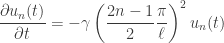
A quick way to understand the behaviour of this equation is to take a spatial Fourier transform, which changes the spatial derivative $\nabla^2$ to a simple multiplication by the wavevector modulus:

$\displaystyle{\frac{\partial \tilde{u}}{\partial t} +\gamma|k^2|^2 \tilde{u} = 0}$

where $\tilde{u}$ is the Fourier transform of $u$ . Solving this equation in time, we have

$\displaystyle{ \tilde{u}(k, t) = \tilde{u}_0(k)e^{-\gamma|k^2|t} }$

for some initial spatial conditions $\tilde{u}_0(k)$ .

What this tells us is that any particular component $\tilde{u}_k$ of the solution decays in time exponentially. This sounds very similar to Newton’s idea above, which is encouraging. Having probed a little at the heat equation, let’s get our hands dirty and find a concrete solution to the thing.

Solving the heat equation

The above discussion about heat transport between bodies is a bit vague. To firm things up, we’ll consider here two bodies in one dimension of length $\ell$ and temperatures $T_1, T_2 \,\,\,T_1>T_2$ .

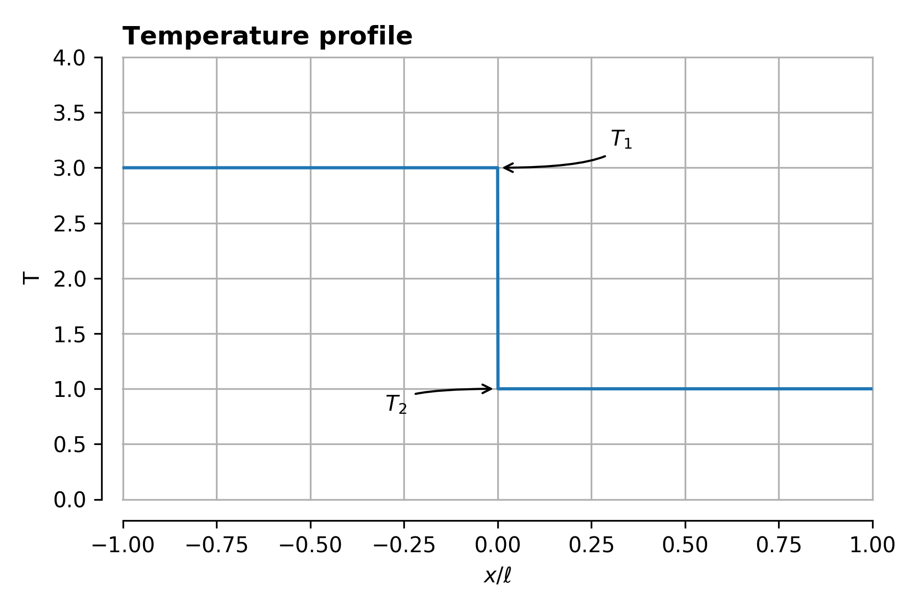
There’s a good reason I’ve picked this initial condition – it makes the following maths quite a bit less tedious. In general, if you’re investigating a general question rather than a specific situation, always pick the simplest possible question to answer. You’ll have an easier time, and look just as smart at the end of it!

Specifically then, knowing a bit about what the answer will end up being, we can represent the solution as

$\displaystyle{u(x, t) = \frac{T_1 + T_2}{2} + \sum_n u_n(t)\sin(k_n x)}$ .

For $t \rightarrow \infty$ , we know that the temperature will even out and so $u(x, \infty) = (T_1 + T_2)/2$ . At all other times, due to the symmetry of the initial conditions, the discrepancy about this average will be an odd function, which can always be represented as a sum of $\sin$ functions. To allow the solution to change with time, we need to make the coefficients of these functions $u_n$ vary with time.

Now as represented above, $k_n$ can take any value. We’ll cut this down by imposing some boundary conditions, namely that heat energy cannot flow out of the region $-\ell < x < \ell$ , and so therefore the derivative of $u(x,t)$ is zero at the boundary for all $t$ .

To achieve this, we only allow

$\displaystyle{k_n = \frac{2n - 1}{2}\frac{\pi}{\ell}}$

so the solution we are investigating looks like

$\displaystyle{u(x, t) = \frac{T_1 + T_2}{2} + \sum_n u_n(t)\sin\left(\frac{2n - 1}{2}\frac{\pi x}{\ell}\right)}$

Progress! All that is left to do is to find the infinite different $u_n(t)$ .

Initial conditions

This might sound like we’ve gotten nowhere, so let’s start with something we definitely know because we insisted upon it – the initial conditions of the problem.

The temperature distribution starts out as some function, call it $f(x)$ . We want to find the set of $u_n(0)$ which cause the summation above to converge to $f(x)$ . The trick here is to use a property of the ‘base functions’ we’re using called orthogonality. There are general methods of constructing such orthogonal basis sets, here the family of sinusoids will do just fine.

Let’s first denote

$\displaystyle{s_n(x) \equiv \sin\left(\frac{2n - 1}{2}\frac{\pi x}{\ell}\right)}$

Then the equation to solve is

$\displaystyle{f(x) = \frac{T_1 + T_2}{2} + \sum_n u_n(0)s_n(x)}$

Now the trick – multiply both sides by $s_m(x)$ and integrate from $-\ell$ to $\ell$ :

$\displaystyle{\int_{\ell}^{\ell} f(x)s_m(x)\,\text{d}x = \int_{\ell}^{\ell} \frac{T_1+T_2}{2}s_m(x) \,\text{d}x + \sum_nu_n(0)\int_{\ell}^{\ell}s_n(x)s_m(x)\,\text{d}x}$

All the sinusoids are odd functions, so the first term disappears. The second term can be show to be

$\displaystyle{\int_{\ell}^{\ell}s_n(x)s_m(x)\,\text{d}x =\left\{ \begin{array}{ll}\ell&n = m\\0&n \neq m\end{array}\right.}$

This is precisely the definition of orthogonal – all of the ‘basis functions’ $s_n(x)$ contribute independently to the value of the integral above. This is very useful, as we can then look at each term in the summation in turn.

One can do the integrals, knowing of course what $f(x)$ is, and the result is

$\displaystyle{u_n(0) = \frac{2(T_2 - T_1)}{\pi(2n-1)}}$

With this result and the orthogonality trick in hand, we can finally solve the heat equation.

The solution

Let’s take the expression for $u(x,t)$ above and substitute it into the heat equation:

$\displaystyle{\sum_n \frac{\partial u_n(t)}{\partial t}s_n(x) + \gamma \sum_n \left(\frac{2n - 1}{2}\frac{\pi}{\ell}\right)^2 u_n(t) s_n(x) = 0}$

Using again the orthogonality of $s_n(x)$ , we have

$\displaystyle{\frac{\partial u_n(t)}{\partial t} = -\gamma \left(\frac{2n - 1}{2}\frac{\pi}{\ell}\right)^2 u_n(t)}$

$u_n(t) = u_n(0)\exp\left(-\gamma \left(\frac{2n - 1}{2}\frac{\pi}{\ell}\right)^2 t \right)$

And that’s it! Note by the way how similar this solution looks to the Fourier transformed heat equation at the beginning – all we have done is go through a slightly more laborious Fourier transform. Technically we have just expressed our solution in a particular orthogonal basis set. If the basis set is the sinusoids, then that decomposition is just a Fourier transform.

Plugging everything together in one beastly expression, the answer is

$\displaystyle{u(x,t) = \frac{T_1 + T_2}{2} + \sum_n \frac{2(T_2 - T_1)}{\pi(2n-1)} \exp\left(-\gamma \left(\frac{2n - 1}{2}\frac{\pi}{\ell}\right)^2 t \right) \sin\left(\frac{2n - 1}{2}\frac{\pi x}{\ell}\right) }$

Phew. Let’s plot this out and check it looks as we expect:

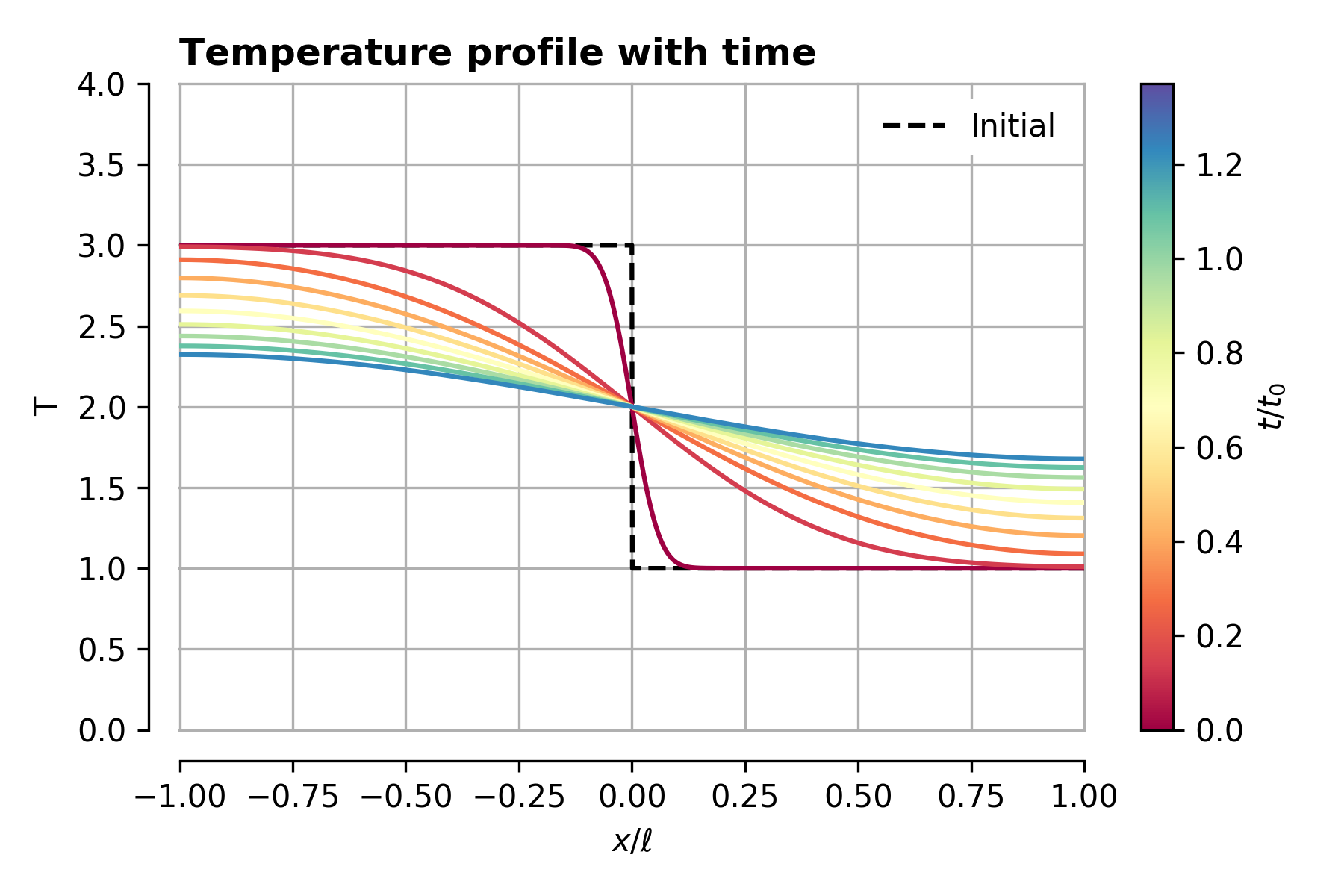
I’ve written time here in terms of a characteristic cooling time taken from the exponential term:

$\displaystyle{t_0 = \frac{4\ell^2}{\gamma\pi^2}}$

We see from the above that after approximately one cooling time, the temperature profile has mostly flattened out.

We can also observe that the gradient of the temperature goes to zero at the edges of the plot – this is because we forced there to be no heat flux from the edges of the solution domain.

The cooling process

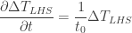
With a solution in hand, we are now much better equipped to answer questions about the cooling process. For example, we can straightforwardly calculate the average temperature excess as a function of time of the leftmost body initially at temperature $T_1$

$\displaystyle{\Delta T_{LHS}(t) = \frac{4(T_1 - T_2)}{\pi^2}\sum_n\frac{1}{(2n-1)^2}\exp(-(2n-1)^2t/t_0)}$

Note something about this expression – it is a sum of decaying exponential functions, but the amplitudes of the functions decay very quickly like $n^2$ , and the rate of decay sharply increases with $n$ like $e^{-n^2}$ . We can therefore concentrate on the first term only, so that

$\displaystyle{\Delta T_{LHS} \approx \frac{4(T_1 - T_2)}{\pi^2}e^{-t/t_0}}$

or differentiating,

$\displaystyle{\frac{\partial \Delta T_{LHS}}{\partial t} = \frac{1}{t_0}\Delta T_{LHS}}$

And there is Newton’s less famous fourth law all over again. More importantly, how does it stack up to the actual solution of the heat equation?

It is actually pretty good! Beyond around half a cooling time there is very little difference, with a larger discrepancy at the beginning of the process.

Whether or not Newton’s law is a good estimate or not ultimately comes down to how the heat energy is initially distributed. If the first term in the sum for $\Delta T_{LHS}$ dominates, then the sum is well approximated by a single exponential term. This can happen, say, when $u_1(0) \gg u_2(0)$ , or that ‘low frequency’ terms in the expansion of the initial conditions are large compared to ‘high frequency’ terms. This in turn happens when the initial distribution of temperature is very smooth, without sharp discontinuities and large temperature gradients. This is the case for most macroscopic objects under normal conditions, and so Newton’s law is usually pretty good.

This is all good news for me, as I (and soulmate Newton) am ultimately vindicated a decade on. Now, what about that teacher who complained about my handwriting…

See the (very basic) notebook here

https://github.com/jasmcole/Blog/blob/master/Heat%20Equation/HeatEqu.ipynb

Almost looks like work

Newton’s 4th Law

Newton’s law

Approximate behaviour

Solving the heat equation

Initial conditions

The solution

The cooling process

Leave a Reply Cancel reply

Newton’s law

Approximate behaviour

Solving the heat equation

Initial conditions

The solution

The cooling process

Share this:

Like this:

Related

Leave a Reply Cancel reply