The perfect speed bump

Sitting in traffic in the middle of London gives you a lot of time to think. Here’s a fun problem born entirely of frustration sat waiting to cross the Hammersmith bridge.

Let’s play a thought experiment. You, dear reader, are a highways technician tasked with installing a new speed bump on a road near your house. Your boss has given you a precise volume of concrete to use, but you know you’ll be going over this bump often enough that it will be a problem. Given your load of concrete, what shape should you make the speed bump to minimise your misery?

Let’s break it down. You’re in a car going at horizontal speed $v_0$ , and you hit a speed bump of width $2\ell$ and cross-sectional area $A$ . The shape of the bump is described as a function $y(x)$ – see the diagram below:

Some things we can deduce – your speed at any point is determined by the shape of the curve $y(x)$ . By conservation of energy, $mv(x)^2/2 + mgy(x) = mv_0^2/2$ . Therefore we have

$v(x) = \sqrt{v_0^2 - 2gy(x)}$

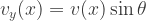
If we also assume that the car wheel stays stuck to the speed bump, then the angle your velocity vector makes with respect to the ground at any point is given by

$\tan\theta = {\displaystyle \frac{\text{d}y}{\text{d}x}}$

and the velocity in the $x$ and $y$ directions is

$v_x(x) = v(x)\cos\theta$

$v_y(x) = v(x)\sin\theta$

With these ground rules laid down, let’s turn to what we should be optimising for. The thing that makes speed bumps unpleasant is the amount of vertical acceleration – that’s the jolt you feel as you go over one.

We’d like to minimise acceleration in the $y$ direction, over the time we travel over the bump. A mathematically nice way to minimise the absolute value of a function is to minimise the square of the function, i.e. what we want to calculate is

${ \displaystyle \int} \left(\frac{\text{d}v_y}{\text{d}t}\right)^2 \, \text{d}t$

and then minimise it.

The problem is that we don’t have $v_y(t)$ , we have $v_y(x)$ , so there’s a bit of rearranging to do.

Note that the time it takes the car to move horizontally $\delta x$ is $\delta x / v_x(x)$ . Then the vertical acceleration is

$a_y(x) = {\displaystyle v(x)\cos\theta \frac{\partial v_y}{\partial x} = \sin\theta\frac{\partial v}{\partial x} + v\cos\theta\frac{\partial \theta}{\partial x}}$

Using the shorthand $y' = dy/dx$ , we have

$a_y(x) = {\displaystyle \frac{v}{1+y'^2}\left(y'^2\frac{\partial v}{\partial y} + \frac{vy''}{1 + y'^2}\right)}$

You might be thinking that this isn’t a particularly elegant looking formula to work with, and you’d be absolutely right. To continue with the analytical effort (as opposed to numerical – see later), let’s start approximating.

First, most speed bumps satisfy $y < v_0^2/2g$ , i.e. most cars are going fast enough that they don’t slow down much due to the change in height going over the bump. We can therefore set $v(x) \approx v_0$

Secondly, the slope of the bump will be assumed to be weak so $y' \ll 1$ – this effectively means that we will approximate $\tan\theta \approx \sin\theta \approx \theta$ .

Plugging these assumptions through, and converting the integral over time into one over position, we end up trying to minimise the following integral:

$\int v_0^3y''^2 \, \text{d}x$

The mathematically astute amongst you will realise that the trivial solution is to have $y'' = 0$ , or the speed bump taking the form of a straight line. This is indeed a solution, as the vertical acceleration is zero at all times. If we add the boundary conditions that $y(\pm\ell) = 0$ , then the solution is no speed bump at all! In this case the highways technician would achieve their goal, but probably get sacked in the process.

Of course, we’ve forgotten to include the fact that the cross-sectional area of the speed bump needs to stay fixed, or

$\int_{-\ell}^{\ell} y(x) \, \text{d}x = A$

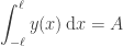
This is a constraint on the minimisation problem, and must be included.

The generic way to include such constraints is to minimise a linear combination of the problem and constraint, i.e. we should minimise

$\int_{-\ell}^{\ell} v_0^3y''^2 + \lambda y\, \text{d}x$

where $\lambda$ is an arbitrary constant which we would later adjust to enforce the area constraint.

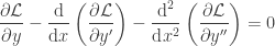
To actually do the minimisation, note that the end points of the integral are fixed, and the solution we are trying to find is a simple scalar function of the integration variable, in which case the answer comes from the Euler-Lagrange formula. Writing the integral as

$\displaystyle \int \mathcal{L}(x, y', y'') \, \text{d}x$

the solution is given by

$\displaystyle \frac{\partial \mathcal{L}}{\partial y} - \frac{\text{d}}{\text{d}x}\left(\frac{\partial \mathcal{L}}{\partial y'}\right) - \frac{\text{d}^2}{\text{d}x^2}\left(\frac{\partial \mathcal{L}}{\partial y''}\right) = 0$

or explicitly in this case

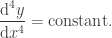
$\displaystyle \frac{\text{d}^4y}{\text{d}x^4} = \text{constant.}$

This is pleasingly simple! The general solution is a 4th-order polynomial

$\displaystyle y = ax^4 + bx^3 + cx^2 + dx + e$

which we need to apply some boundary conditions to to find.

Firstly, let’s make the speed bump symmetric, so the odd powers disappear.

Secondly, let’s enforce that $y(\pm\ell) = 0$ , and also $y'(\pm\ell) = 0$ .

Finally, let’s make the area under the curve from $-\ell$ to $\ell$ A.

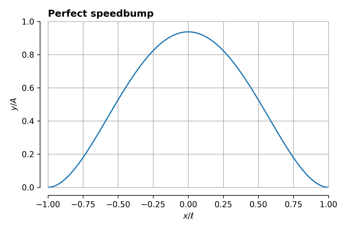
Then the solution is

$\displaystyle y = \frac{15}{16}\frac{A}{l}\left( \left(\frac{x}{\ell}\right)^4 - 2\left(\frac{x}{\ell}\right)^2 + 1 \right)$

or plotted,

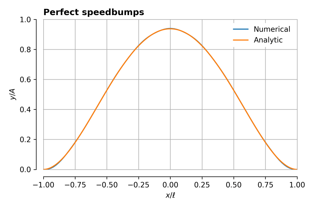
While it is always very pleasing to come up with a simple analytical solution to a problem, we should remember that this is only an approximation. Is it possible to do better than this going beyond pen and paper?

I had a decent go at this, writing a gradient-descent optimiser which started with the analytic shape and optimised according to the exact equations above. The results were… not very different. You can see below that the optimal shape is slightly flatter at the edges and slightly taller overall, but otherwise very close to the solution we already found.

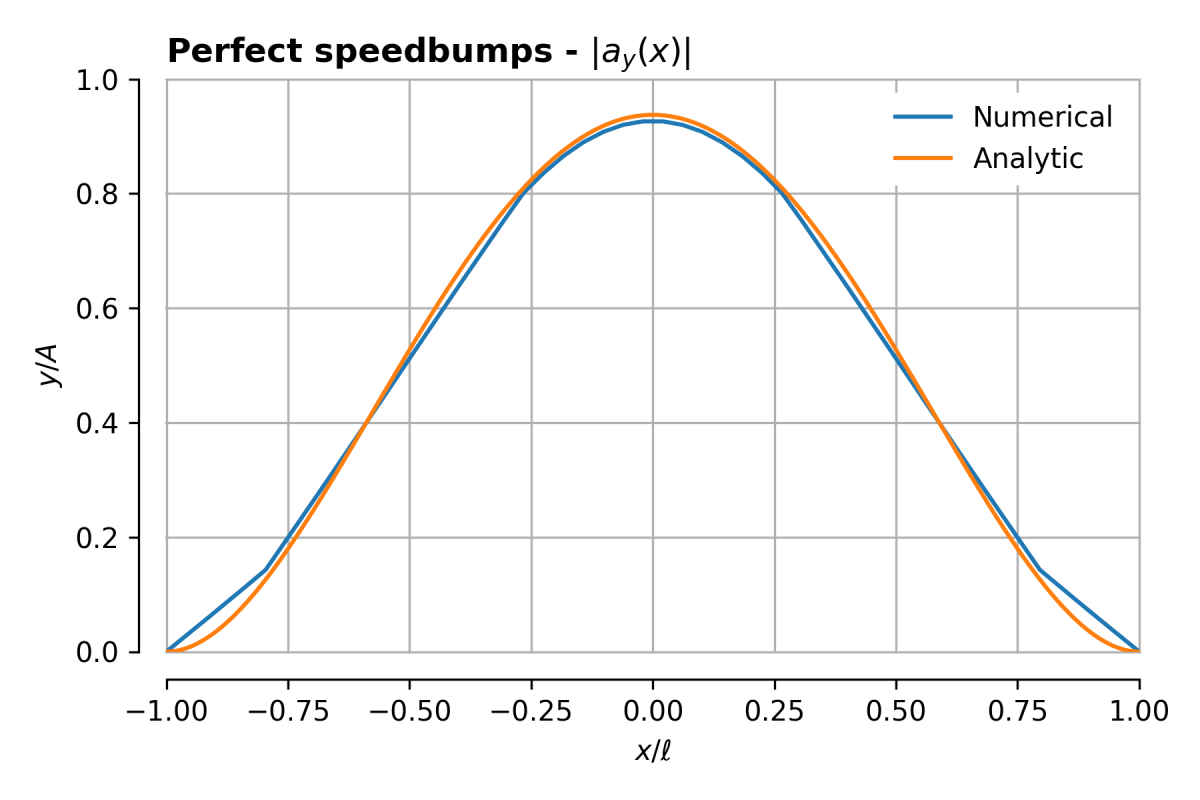
Being a numerical method, it is simple to change some of the other assumptions above. What if we minimise the integral of $a_y$ rather than $a_y^2$ ? As you see below, this results in a slightly wider and shorter speedbump, but overall rather similar in shape.

I’m quite fond of this post as it managed to generate a fair amount of work from an observation I’m sure many people have idly made while stuck in traffic. As the great Adam Savage once said, the only difference between science and mucking about is that science is written down. I think this post therefore qualifies!

7 thoughts on “The perfect speed bump”

Pierre says:

October 9, 2018 at 1:47 pm

One could argue that the aim of a speed bump is to limit the maximum speed of cars going over it. Would it be possible to search for a solution that would have minimal cost below the speed limit but increase very rapidly once you reach this value ?

LikeLike

1. jasmcole says:
  
  October 9, 2018 at 4:44 pm
  
  You’ve been reading the literature! This seems to be exactly what people have thought about before, e.g.
  https://www.tandfonline.com/doi/abs/10.1080/08905459708945498
  The solution ends up looking like a double-hump, presumably exploiting the resonance characteristics of the car-wheel system modelled in that paper.
  
  LikeLike
  
  1. Matt says:
    
    October 11, 2018 at 4:24 am
    
    I had a go at maximising for y acceleration, just for fun. I wound up with a crazy high order non-linear ODE and left it there. I wonder if the double-hump is a solution for the ODE.
    
    Great post. I very much enjoyed it.
    
    LikeLike
  2. jasmcole says:
    
    October 15, 2018 at 11:08 am
    
    Presumably there is no maximum for the average acceleration – just keep making the solution spikier? If you have something set up though, it’s fun to try different boundary conditions, i.e. bump heights and slopes at edges. In particular, if you don’t constrain the derivative at the edges, you end up with something that looks a lot like part of a sinusoids.
    
    LikeLike
John Doe says:

October 10, 2018 at 8:03 pm

Two small remarks:
* in your first equation for $a_y(x)$ , the last equality is incorrect: you miss the initial $v(x) \cos(\theta)$ factor to the rightmost part ;
* the general equation you give for the Euler-Lagrange equation is not correct: the signs should alternate, that is it should be a $+$ sign before the second derivative $\frac{\mathrm{d}^2}{\mathrm{d} x^2}$ part.
Note that none of that change the overall results and other equations of this post.

LikeLike

1. jasmcole says:
  
  October 27, 2018 at 6:45 pm
  
  Thanks for the comments! I must admit, I spotted the first of your points and assumed no one would notice – thank you for proving we wrong 🙂 On the second, thanks for the correction. I last studied the calculus of variations ~8 years ago, but that’s no excuse for sloppiness!
  
  LikeLike
  
tobi says:

October 26, 2018 at 9:05 am

This is awesome.

Another way to numerically solve this would be to use a single step of reinforcement learning with actor critic. The agent outputs a curve shape (e.g. 100 floats). The critic learns to approximate the utility function. The gradient from the critic is pushed into the actor to maximize utility. The ground truth reward is generated by numerically evaluating the shape possibly using a physics simulation.

LikeLike