It’s winter again in the UK which means even more rain than usual, often accompanied by oddly-named storms. Sadly this also occasionally means flooding for many parts of the country, a fact which I usually watched with some detachment from the other (safer) side of a news report. This year is different – I have bought a house quite near the river Avon, which makes the issue more immediate. I suppose I could campaign for flood defences, or petition my new local MP, but for now let’s stick to what I know: data and maths.

Environment data API

For those readers not in the UK, the two most recent storms were called Ciara and Dennis (named alphabetically).

For reference, here’s the river in question during storm Dennis – fortunately my new house is some way behind the camera:

This picture prompted an investigation of the river level reporting systems in the UK, which are surprisingly great – check out how detailed the flood risk map is:

https://flood-warning-information.service.gov.uk/long-term-flood-risk/map

or the density of monitoring stations:

https://flood-warning-information.service.gov.uk/river-and-sea-levels

All of which is backed by an API which updates every 15 minutes:

https://environment.data.gov.uk/flood-monitoring/doc/reference

There are a few limitations to the API – accessing information about a given monitoring station is limited to the last 28 days, and the only other option for readings older than that is historical data for the entire country.

River level data

Nevertheless, I downloaded all 18 GB of their historical data and filtered it for the few megabytes I was interested in:

import datetime
from datetime import date, timedelta
import os

start_date = date(2019, 1, 1)
end_date = date(2020, 2, 23)
delta = timedelta(days=1)

while start_date <= end_date:
    today = start_date.strftime("%Y-%m-%d")
    
    cmd = 'curl -s http://environment.data.gov.uk/flood-monitoring/archive/readings-' + today + '.csv | grep -e <Some reading> -e <Another reading> > ' + today + '.csv'
    
    os.system(cmd)
        
    start_date += delta

The river level over the previous year looks like this:

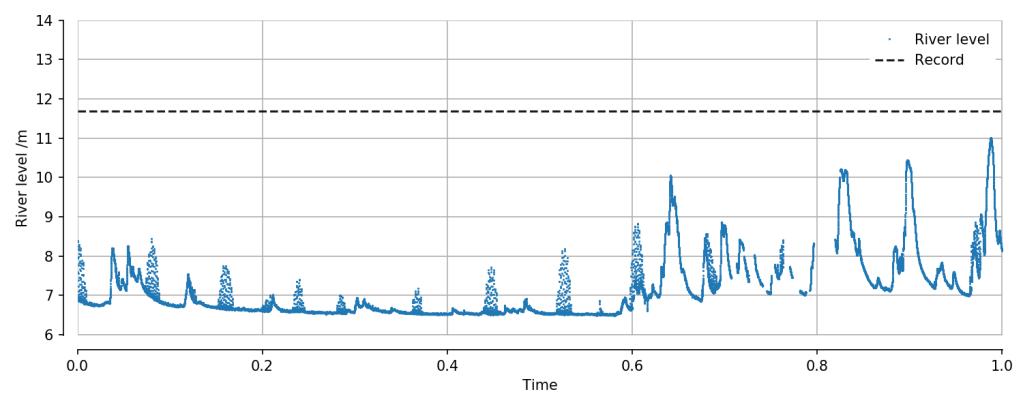
While there are a few gaps, the coverage is pretty good! There are a few places where the river level spikes at 6-hourly intervals:

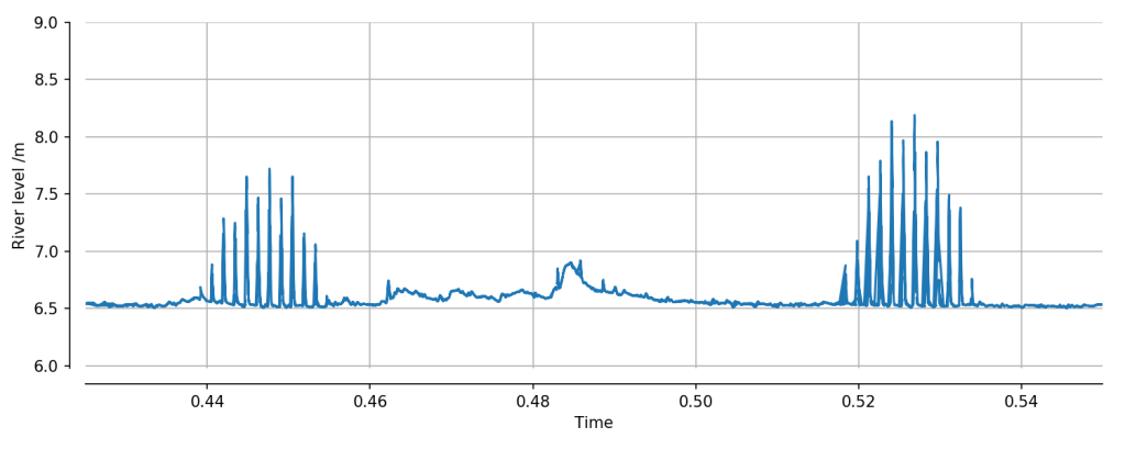
Apparently, after having spoken to someone involved in the API, this is due to sluice gates opening upstream in an attempt to manage river levels elsewhere – this particular measuring station is just downstream of the confluence of two rivers, and as such is probably an important control point.

To put the recent storms in context, lets integrate the timeseries plot sideways to get a distribution of river levels:

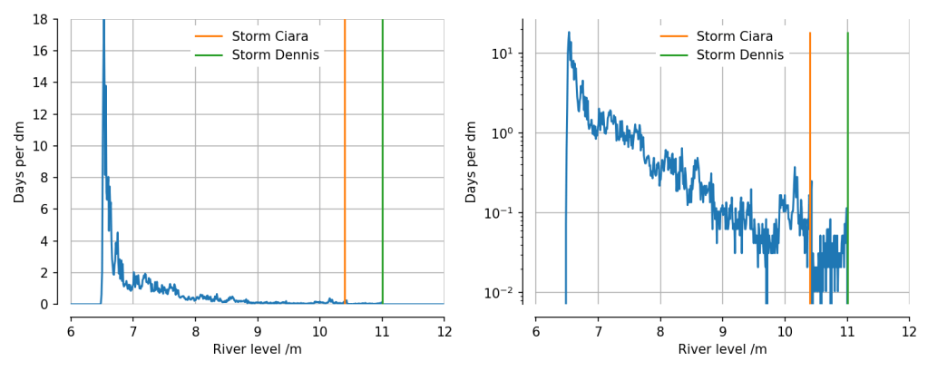
With the following CDF

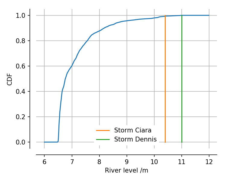
These plots make it evident that Ciara and Dennis were pretty exceptional events – over the last 341 days, storm Dennis produced the highest river level in the dataset, with storm Ciara only slightly behind (river levels of 11m and 10.4m respectively).

It gets interesting when we look at the recorded rainfall (from the same API) in conjunction with the river levels:

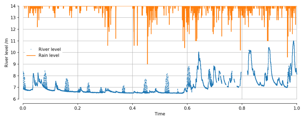
The UK being what it is, there is pretty regular rainfall throughout the year, and in this case there are some points where the rainfall was even higher than that seen during storm Dennis – so why were these two storms so destructive?

Most news reports indicated that the problem was rain falling on already-saturated ground, meaning the rivers collected more of the rain than usual. Let’s whip up a simple model for this situation and see what the implications are.

Modelling considerations

Let’s keep things simple, and take our model universe to be zero-dimensional and consist entirely of rain, groundwater, and a river. This means ignoring the time taken for water to flow from place to place, but as we’ll see later some temporal delay comes for free.

There are then just 3 scalar quantities to consider:

• Rainfall as a function of time
• Groundwater level as a function of time , with a posited maximum level of
• Water level as a function of time , with a posited normal level of

Then there are a couple of tweakable parameters

• The rate at which groundwater drains into the river – this must be proportional to the groundwater level
• The rate at which rain flows into the groundwater – the flow must also go to zero when , and be a maximum when
• The rate at which the river level falls to it’s natural level, due to the difference in inflow rate (presumed constant) and water leaving this section of the river ().

These interactions together look like:

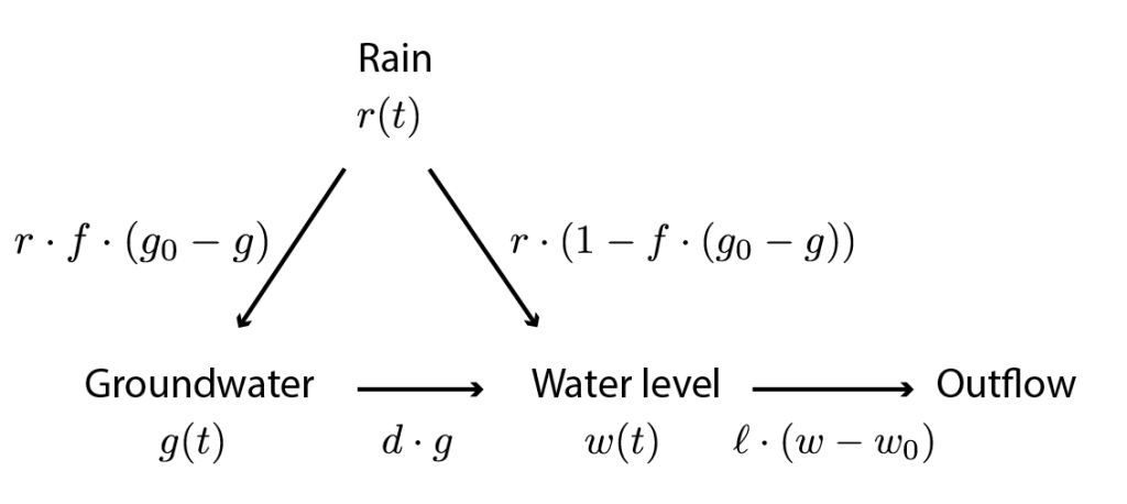
which you can write as a pair of coupled ODEs:

Let’s get a quick intuitive feel for the behaviour of these ODEs.

Under constant rainfall, we can solve the equation for the groundwater assuming it starts at zero:

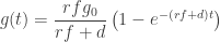
i.e. it fills up to a constant level

which asymptotes to as (also known as the British Winter limit).

It’s a bit trickier to solve the second equation, but in the limit you get that

which makes sense – higher rainfall and lower outflow rates raise the equilibrium water level.

Solving the model

Enough maths, let’ solve this numerically like adults (and people who forgot all of their maths).

Solving the ODEs with all parameters set to 1 as God intended, we get solutions of the expected form:

As predicted, both levels tend to a constant. Note something interesting though – the river water level rises to a peak more slowly than the groundwater level. This model has a delay built-in even for constant rainfall, due to the dynamical interplay between the groundwater and river levels.

To illustrate the sequential-storms problem, let’s look at a worst-case scenario, where there is no groundwater drainage at all, and two short bursts of rain:

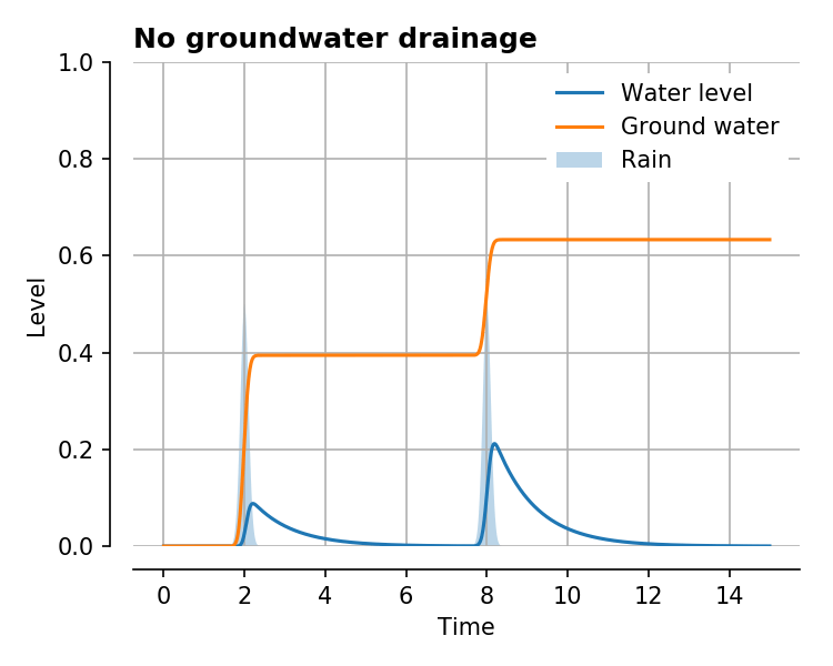
In this case the exact same amount of rain is deposited (), but the rise in river level in the second case is double that of the first. This is because the groundwater level is already high by the time the second burst of rainfall comes, and can’t absorb as much of the rain. Intuitively obvious, but it’s always nice to have an equation to back you up.

If we instead turn on groundwater drainage, there is no extra bump in river water level:

Finally, how does this simple model fare against actual data? Well, given enough arbitrary parameter-tweaking, not terribly – the simulation is on top, with the real data below. The rainfall used as the input to the simulation is interpolated from the recorded rainfall:

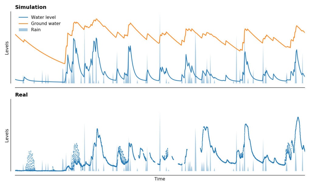
We predict (just about) that the peak due to storm Dennis is slightly higher than that of storm Ciara, and lots of the smaller features are a good match too. It’s a bit curious that the large amount of rain towards the start doesn’t case a big river level increase in real life, though you can see that there is some energetic sluice-gating going on around then, so perhaps the fine people in charge of our rivers worked some magic there.

As climate change really starts to show its teeth, it’s a sad fact that flooding events like those seen recently will become more and more common. While the UK government suffers from a great many flaws, I am encouraged that it seems to have its shit together when it comes to timely information about flooding and river levels, which will undoubtedly come in useful in the years ahead.

Especially if you bought a house on a bloody river.