On which shaped planet am I the heaviest?

Continuing on from my last post concerning optimisation and Lagrange multipliers, I came across a neat little paper on the arXiv here, which asks and answers the question: what shape should a planet be to maximise the gravitational force at a given position? This is a fun problem, solved using an extension of the techniques from the last post, namely the use of Lagrange multipliers to optimise a function given some constraint.

Let’s set some things down before we begin. Assume in the diagram below that we are stood at the pole of an arbitrarily-shaped planet, marked with the red dot. By symmetry, the planet will be cylindrically symmetric, but may have a varying profile. We should then use a cylindrical coordinate system to describe the surface of the planet – call this radius $r(z)$ as a function of depth below our feet $z$ :

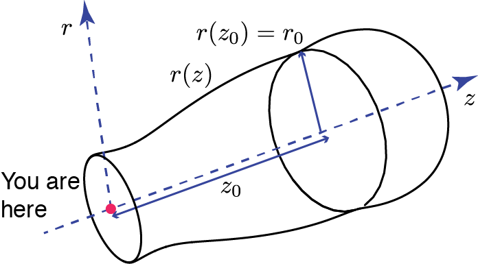
We want to calculate the total gravitational force caused by a planet of this shape at our position. To do this, let’s split up the planet into a series of disks. Suppose the disk at a distance $z_0$ has a radius $r(z_0) = r_0$ . Also suppose it has density $\rho$ and thickness $\Delta z$ , which we assume is very small. Referring to the diagram below, we can calculate the gravitational force caused by the small mass element coloured in red. The gravitational force exerted on us is depicted by the red line. Due to symmetry, only the component along the $z$ -direction will matter, the other components will cancel out when we add the rest of the disk. Once we find the force due to this small component, we can integrate over the rest of the disk.

It has dimensions $da \times ad\phi \times \Delta z$ , so has mass $dm = \rho\Delta z a da d\phi$ . It is a distance $d = \sqrt(z_0^2 + a^2)$ from us, so the magnitude of the force is given by Newton as

$dF_{disk} = \frac{GM_1M_2}{d^2}$

or equivalently the acceleration

$dA_{disk} = G\rho\Delta z \frac{a da d\phi}{z_0^2 + a^2}$

Finally we should include the fact we only need the $z$ -component of the acceleration, so we multiply by $\cos\theta = z_0/d$ . We can also integrate trivially over $\phi$ while we’re at it:

$dA_{disk} = 2\pi G\rho\Delta z z_0\frac{a da}{(z_0^2 + a^2)^{3/2}}$

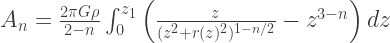
The total acceleration is then given by integrating over $a$ to the edge of the disk:

$A_{disk} = 2\pi G\rho\Delta z z_0 \int_0^{r_0} \frac{a}{(z_0^2 + a^2)^{3/2}} da$

$A_{disk} = 2\pi G\rho\Delta z\left(1 - \frac{z_0}{\sqrt{z_0^2 + r_0^2}}\right)$

To get the force from the entire planet then, we continue this integration to the rest of the $z$ -coordinate, remembering that the radius of each infinitesimal disk may change:

$A = 2\pi G\rho \int_0^{z_1} \left(1 - \frac{z}{\sqrt{z^2 + r(z)^2}}\right) dz$

Now we’ve defined in our co-ordinate system that we’re standing at the origin, so the planet must begin at $z = 0$ . However we haven’t defined yet the endpoint of the planet $z_1$ – it could continue on indefinitely. We need to add a constraint then, otherwise we could keep making the planet bigger and bigger to increase the gravitational force. The constraint we need is that of constant mass – we are only interested in the relative shape of the planet. This is a constraint on the function $r(z)$ through the definition of the mass $M$ of the planet (assuming cylindrical symmetry):

$M = \pi\rho\int_0^{z_1}r(z)^2 dz$

Now this looks familiar – if we want to optimise something subject to a constraint, we should aim to optimise some linear combination of the quantity of interest and the constraint. In this case we should be optimising

$L[r(z)] \equiv A[r(z)] - \lambda M[r(z)] = \int_0^{z_1} \mathcal{L} dz$

where $\lambda$ is the Lagrange multiplier and $\mathcal{L}$ is analogous to some Lagrangian density

$\mathcal{L} = 2\pi G \rho \left(1 - \frac{z}{\sqrt{z^2 + r(z)^2}}\right) - \lambda\pi\rho r(z)^2$

Now in the above I’ve been notating these objects with square brackets to distinguish them from functions. Functions take a number and return another number. These things are functionals, which take a function and return a number. We are now trying to find a function which minimises a functional.

From the Euler-Lagrange equation we know that in order to find an extremum of this functional, the required function $r(z)$ solves the equation:

$\frac{\partial \mathcal{L}}{\partial r} - \frac{d}{dz}\left(\frac{\partial \mathcal{L}}{\partial r'}\right) = 0$

where $r' = dr/dz$ . This reduces to $\partial \mathcal{L}/\partial r = 0$ , or

$\frac{Gz}{(z^2 + r^2)^{3/2}} = \lambda$

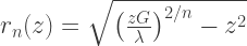
We can rearrange this expression to get our planet’s shape:

$r(z) = \sqrt{\left(\frac{zG}{\lambda}\right)^{2/3} - z^2}$

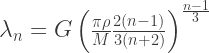
Now we’re almost done – we just need to fix the unknowns $z_1$ and $\lambda$ . For the first, note that by definition $r(z_1) = 0$ , or equivalently

$z_1 = \sqrt{\frac{G}{\lambda}}$

We can then substitute everything into our equation for the mass of the planet:

$M = \pi\rho\int_0^{\sqrt{G/\lambda}}\left(\frac{zG}{\lambda}\right)^{2/3}- z^2 dz \Rightarrow \lambda = G\left(\frac{4\pi\rho}{15M}\right)^{2/3}$

Finally, we have a complete solution, which is plotted below along with a spherical planet of the same mass.

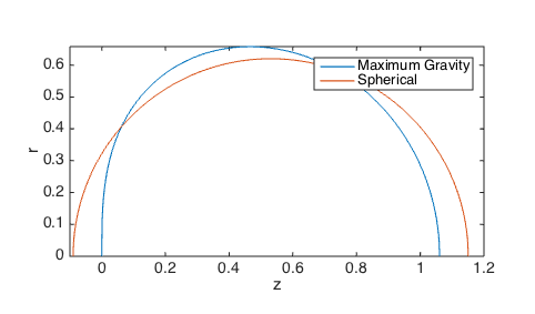
We have fixed the mass and density of our planet, and we may notice that we have implicitly defined a lengthscale $l_0 = \sqrt{G/\lambda} = (15M/4\pi\rho)^{1/3}$ . Move to dimensionless coordinates then, where we scale by this lengthscale $\hat{r} = r/l_0, \hat{z} = z/l_0$ , and we end up with

$\hat{r} = \sqrt{\hat{z}^{2/3} - \hat{z}^2}$

In this co-ordinate system the equation of a perfect sphere would be

$\hat{r} = \sqrt{0.5^2 - (\hat{z} - 0.5)^2} = \sqrt{\hat{z} - \hat{z}^2}$

so the act of maximising the gravitational force has squashed a circular planet up towards the observation point, by modifying the exponent of the first term in the equation for $r(z)$ .

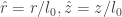
Lets draw this planet a little more intuitively, in these normalised coordinates:

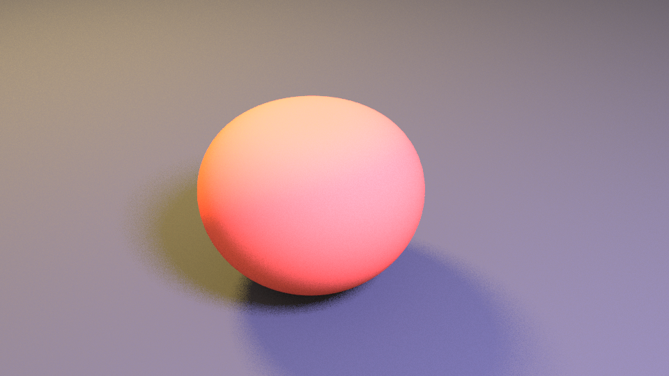Here I’ve written a Python script for Blender to create and light the correct geometry. The $z$ -coordinate is now vertical (confusingly!), and the radial coordinate transverse. The top of this orb represents $\hat{z} = 0$ .

I’d like to be able to generalise this model to explore different planetary shapes. A simple thing to do is to see what happens when we change the way gravity spreads out. The current model for gravity suggests an inverse-square law, so the force exerted by a mass scales with radius like $1/r^2$ . There are some theories which predict a departure from this scaling at small or large scales though, so let’s play around a bit. Assume the force of gravity in $n$ -dimensional space scales like $1/r^{n-1}$ . Going through the above derivation again, we then have the generalised results

$A_n = \frac{2\pi G\rho}{2-n} \int_0^{z_1} \left(\frac{z}{(z^2 + r(z)^2)^{1 - n/2}} - z^{3-n}\right) dz$

$\mathcal{L}_n = \frac{2\pi G\rho}{2-n}\left(\frac{z}{(z^2 + r(z)^2)^{1 - n/2}} - z^{3-n}\right) - \lambda\pi\rho r^2$

$r_n(z) = \sqrt{\left(\frac{zG}{\lambda}\right)^{2/n} - z^2}$

$z_{1,n} = \left(\frac{G}{\lambda}\right)^{\frac{1}{n-1}}$

$\lambda_n = G\left(\frac{\pi\rho}{M}\frac{2(n-1)}{3(n+2)}\right)^{\frac{n-1}{3}}$

I’ll leave those derivations as an exercise for the terminally bored (it’s simple and only a little tedious). What’s interesting to do is scale the dimensions is each case by the appropriate lengthscale $z_{1,n}$ , and look at how the ‘heavy planet’ changes shape as the force of gravity varies in its behaviour:

It’s important to note that each frame is using a different spatial scaling – in each case the planet has the same volume and mass, but they’ve all been scaled uniformly to fit into the same vertical region.

Switching back to unscaled coordinates, we can see below how the profile of the planets change when gravity operates in different dimensions.

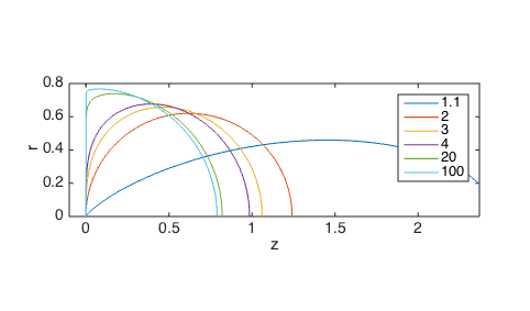
For $n = 2$ , the best solution is actually a sphere again which is nice. For lower dimensions the most important thing is to make sure the force of gravity is mostly along the $z$ -direction so that it doesn’t get cancelled out – the dependence on distance is so weak that its OK to spread the mass out a bit, as long as it’s mostly along the right direction (don’t be fooled by the above plot – all planets have the same volume!).

For higher dimensions, gravity lessens incredibly rapidly with distance so it’s most important to squash as much mass as close to the observer as possible. This leads to the planets becoming a half-sphere shape.

Now this is all very nice, but there is one thing we’ve overlooked, which becomes clear when we actually work out the gravitational force caused by these different planets:

$A_n = 2\pi G\rho\frac{(1-n)}{(n-4)(n+2)}\left(\frac{M}{\pi\rho}\frac{3(n+2)}{2(n-1)}\right)^{\frac{4-n}{3}}$

For $n > 4$ the gravitational force becomes so large so quickly that the material nearest the observer causes the total force to diverge, so we should really restrict our attention to $n < 4$ . As the mass of the planet changes we can see how the total force varies as a function of dimension.

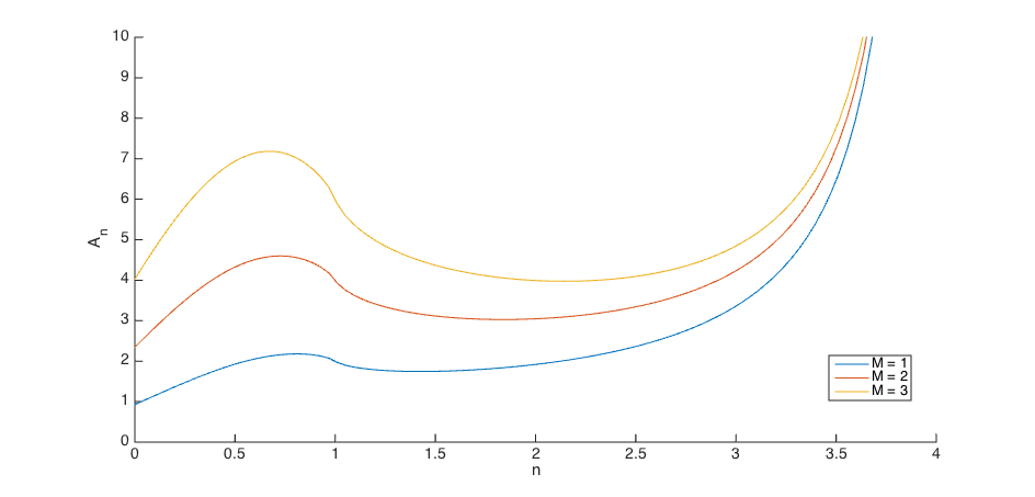For sufficiently massive planets, the gravitational force in lower dimensions can exceed that from a 3-dimensional gravity. While this solution continues for $n < 1$ , we should note that it isn’t actually possible to construct a planet there, as $\lambda$ becomes imaginary (taking a fractional power of a negative number).

Nevertheless, from a simple question we’ve managed to churn out a lot of maths and even a Python script. If you’d like to have a look, you can see it here.

In Blender if you’d like to run the script, open a new .blend file, ensure the selected render is Cycles, open the Python console, and type

filename = 'SCRIPTLOCATION'
exec(compile(open(filename).read(), filename, 'exec'))

There is a line commented out at the end of the script where you can choose where to save the finished render. The rest should be self-explanatory, though if you have any questions feel free to comment below.

Almost looks like work

On which shaped planet am I the heaviest?

Leave a Reply Cancel reply

Share this:

Like this:

Related

Leave a Reply Cancel reply