Fear of heights

I am a short man. I have an even shorter girlfriend. Odds are, any offspring would be short. Odds are, their partners would be similar or smaller in height, especially if they are male. Does this mean I am destined to be the heir to a slowly shrinking troglodyte race, my pristine DNA squirted from troll to troll until it degrades to a corrosive, fetid broth? Let’s put the thesaurus away and have a look.

The model

On average, men are taller than women, though the heights of both populations approximately follow a Gaussian distribution

$P(h) = \exp(-(h - \mu)/2\sigma^2)$

where $P(h)dh$ is the probability of finding a person with height between $h$ and $h + dh$ . For the British population, the relevant parameters (in metres) are around

$\mu_m = 1.75$
$\mu_f = 1.62$
$\sigma_m = 0.23$
$\sigma_f = 0.18$

where I’ve used $m$ and $f$ to distinguish males and females. These define two probability distributions $P_m(h)$ and $P_f(h)$ . The ratio between the average heights of the two populations is then $r = \mu_m/\mu_f \approx 1.08$ . I’d like to model the evolution of these populations through their pairwise interactions (higher-order effects are neglected, notably the infamous three-body problem).

For the sake of simplicity, let’s consider a simple case. A single man and a single woman meet, producing a single male and single female. The parents are then deleted from the population, so the time evolution of the population depends on how the heights of the parents $(h_m, h_f)$ are transformed to the heights of the children $(h'_m, h'_f)$ . Suppose

$h'_{m/f} = \frac{1}{2}(h_m + h_f)$

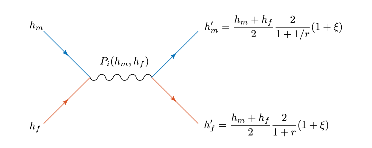
then both children are the same height – the average of the two parents. Let’s physics this up a bit, as we have two things interacting and effectively ‘scattering’ away with different properties. We can represent this as a Feynmann diagram, where blue represents men and orange women (yes, even the default Matlab plot colours suffer from tired gender stereotypes).

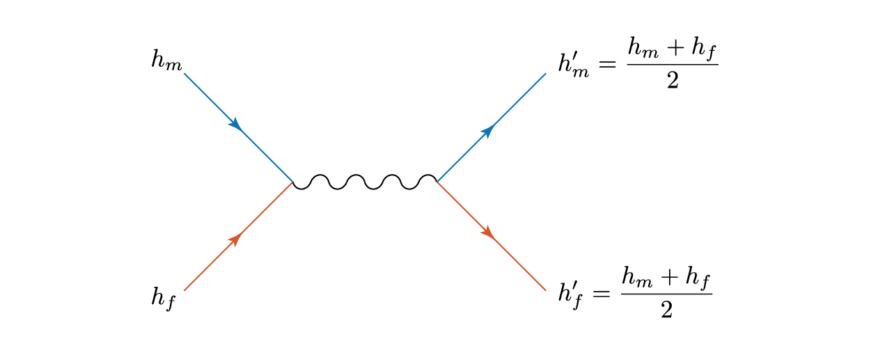
The squiggly line represents the, er, interaction, and the childish amongst you can reinterpret gluons or propagators as you wish.
Total height is conserved in this process, and there is an effective transfer of height

$\Delta h = \frac{h_f - h_m}{2}$

from the man to the woman.

Equal height children

What effect does this have on the population? I simulate a large number of these interactions, randomly picking parents and adjusting their properties as above:

This doesn’t look good – very rapidly the male and female populations converge to the same average height, and the variance of heights within each population is dropping towards zero. This isn’t surprising – if you replace two quantities by their average, the distribution will be losing people at the edges and gaining them in the middle.

Asymmetric children

Let’s adjust our scattering procedure with the assumption that the male child will tend to be taller than the female child, as we observe in the real population:

To see that this is appropriate, consider the average height of the male child averaged over the population (where $\langle\rangle$ represents the averaging operation)

$\langle h_m'\rangle = \frac{1}{1 + 1/r}(\langle h_m\rangle + \langle h_f\rangle)$

which by definition of the mean heights

$\langle h_m'\rangle = \frac{1}{1 + 1/r}(\mu_m + \mu_f)$

So if we take that $\mu_m = r\mu_f$ then

$\langle h_m'\rangle = \frac{r+1}{1 + 1/r}\mu_f = r\mu_f$

and the average male child height should follow the same ratio on average. What does this do to the population evolution then?

Great, the average heights stay pretty much exactly the same as we wanted. By adjusting the $r$ parameter it is also possible to force the population to evolve however you like. For example, what if male children were 50% taller than female children?

However, the populations still don’t resemble what we observe in the real world. The repeated averaging process homogenises the populations in an unrealistic way.

Random children

What we need is a bit of randomness – adjust the scattering procedure so that it reads

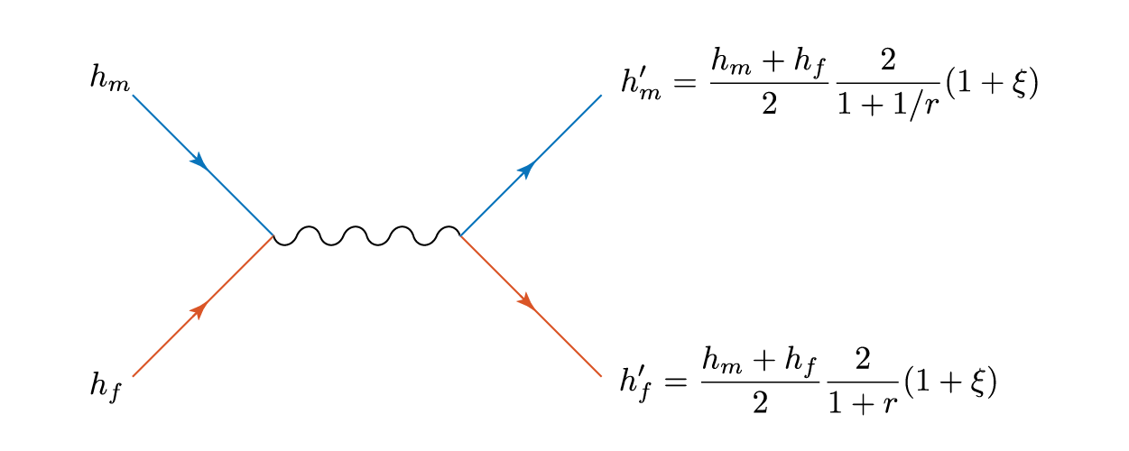
where $\xi$ is a small random number. Unfortunately height is no longer exactly conserved, but we’ll manage. With $\xi$ limited to $\pm 0.15$ the population evolution looks like this:

This is nice, with a bit of gender bias in child heights and a sprinkling of randomness we can reproduce the observed population, and it’s relatively stable.

Interaction probabilities

To start answering the question I posed at the beginning, we’ll need to adjust the final part of the scattering process – the likelihood of interaction $P_i(h_m, h_f)$ :

This is, in general, a function of the heights of the two prospective parents. It could take a number of forms. For example, what if a couple couldn’t tolerate a height difference of more than, say, $\sigma$ centimetres? Then

$P_i(h_m, h_f) = \exp( -(h_m - h_f)^2/2\sigma^2)$

would encourage pairings where the heights of the parents are similar, and discourage pairings with a large different in height. What does this look like in practise?

Here the real winners are short men and tall women, whose populations significantly overlap. They breed themselves out of existence, leaving a lonely population of tall men and short women, each repulsed by the other and breeding slows down.

This is unrealistic, what about the situation where women will tend towards taller men? Here, set $P_i = 0$ for $h_m < h_f$ and the evolution looks like:

In this case the situation is reversed, somewhat counter-intuitively the female population gets taller as it preferentially interacts with taller men. The male population gets shorter as the taller section breeds itself away, In general everyone is pretty happy, except for the initial male population below 1.25 m or so.

PDE model

The above procedure is pretty simple to conceptualise and implement. However, it can be quite slow, especially when the aggregate probabilities of interaction are low. There is another way to look at this process, motivated by physics (naturally).

It is often natural to consider the evolution of a distribution function of some species under the influence of internal and external forces. In plasma physics, for example, the distribution function is that of a particle species over position and velocity. The Vlasov equation then dictates how this distribution function evolves. An important component is the description of scattering processes – when two particles collide they change their velocities, and therefore the shape of the velocity distribution function is changed. One can show that the distribution function is unchanged by scattering (on average) when it attains a Maxwell-Boltzmann form, i.e. is in thermodynamic equilibrium.

It is interesting to consider how our two distribution functions interact through scattering, and under what conditions the populations might be stable. I’ll just think about the simple case here when $\xi = 0$ .

The value of $P_m(h_m')$ is increased when a component at $h_m$ ‘scatters’ into it. It is decreased when a component $h_m'$ is `scattered’ away. The transformation from $(h_m, h_f)$ to $(h'_m, h'_f)$ in the scattering process has zero Jacobian, so is only parametrised by a single degree of freedom. In this case we fix $h_m$ and consider the range of $h_f$ which allow the right scattering, i.e.

$h_m = h_m'\frac{1+r}{r} - h_f$

In the range $h_f, h_f + dh_f$ , the number of available women for the specified interaction is $P_f(h_f)$ . The number of men is $P_m(h_m'\frac{1+r}{r} - h_f)$ . The total number is then found by integrating over the distribution of $h_f$ :

$\int P_f(h_f)P_m\left(h_m'\frac{1+r}{r} - h_f\right)dh_f$

The rate at which $P_m(h_m')$ is depleted is simply the number of men there, i.e. $P_m(h_m')$ (assuming equal probability of interacting with any women, and that the number of women is conserved).

Overall then, we have

$\frac{\partial P_m(h'_m)}{\partial t} = \int P_f(h_f)P_m\left(h_m'\frac{1+r}{r} - h_f\right)dh_f - P_m(h'_m)$

and analogously for the female population

$\frac{\partial P_f(h'_f)}{\partial t} = \int P_m(h_m)P_f\left((1+r)h'_f - h_m\right)dh_m - P_f(h'_f)$

By solving these integro-differential equations numerically, we get the same behaviour as was seem earlier, namely narrowing of the two populations around their respective means.

Hand-waving alert

Notice that the equations above take the form of convolutions. If we Fourier transform with respect to the primed variables then, we have

$\frac{\partial\tilde{P}_m}{\partial t} = \tilde{P}_m(\tilde{P}_f - 1)$

$\frac{\partial\tilde{P}_f}{\partial t} = \tilde{P}_f(\tilde{P}_m - 1)$

(neglecting some constants and lots of rigour). A non-trivial stable solution then arises when the Fourier transform of the two distributions is 1, or when the distributions themselves tend to a delta-function. This is the limiting behaviour we observe in numerical simulation.

I’m not comfortable enough with this technique to take it much farther though, and would therefore welcome corrections or pointers to useful resources.

6 thoughts on “Fear of heights”

Laura K says:

May 18, 2015 at 11:37 pm

Hi there! I love your blog entries – I’ve been following for about a year. I love how you start with a story, and build up the mathematics to reflect some new parameter that is added to make things more realistic.

LikeLike

1. jasmcole says:
  
  May 19, 2015 at 6:50 am
  
  Thanks! The usual procedure is to idly fiddle around with some maths until I get something interesting. Of course I only write about the ones that turn out tractable, so there is some publication bias too 🙂
  
  LikeLike
  
Jacovie says:

June 9, 2015 at 5:02 am

Oh man, I love the Feynmanesque diagramming. This is a fantastic post!

LikeLike

1. jasmcole says:
  
  June 9, 2015 at 6:36 am
  
  Haha, thanks! You have to be a special kind of geeky to start at reproduction and end at Feynman (ish) diagrams.
  
  LikeLike
  
randper says:

August 17, 2015 at 9:36 pm

In the simplest case, how does the height the female population not equal the height of the male population after one generation? In other words, in the case where both offspring have the same height, after one generation the male and female population will have the same samples, however your figures do not show this.

If I am not mistaken. To do this you first sample the initial population. Randomly permute the samples to choose the parents. Then compute the average height to get the heights of the new females and males, and then repeat the procedure.

LikeLike

1. jasmcole says:
  
  September 7, 2015 at 10:12 am
  
  Hi, the reason is that the initial populations contain a broad spread of heights. The two children are the same height for a given set of parents, but over the distribution of parents there will still be many children of different heights after a generation. In each ‘generation’ I pick a sample of parents at random, and replace them with their averages. Doing this enough times the variance in the population is reduced, and I show at the end of the post how the limit of this process is a delta function in height.
  
  LikeLike