In my last blog post I waded through a lot of maths with no pretty pictures to show for it. I’ll redress the balance here and make the pictures extra pretty. The post title alludes to a previous post, and is similar in that I’ll be using mathematics to form interesting 3D objects.

Maxwell…

Last time I went from Maxwell’s equations all the way to the geometric optics limit for a perfect lens. However, I should mention that it is perfectly possible to simulate the behaviour of a lens from a first-principles perspective. In the following video I use the FDTD approach to propagate a pattern of light through a microscopic lens (try to watch in HD):

The lens here is modelled by a semi-spherical cap of dielectric, where the refractive index is larger than 1. Due to Snell’s Law, we see the incoming wavefronts directed towards the optical axis. They come to a focus at the focal length of the lens (defined by the refractive index and the radius of curvature)l before diverging again. The input wavefield is approximately reconstructed at the image plane on the right of the lens. The more exact nature of this kind of simulation reveals a few interesting behaviours, like the distribution of light inside the lens. However it is computationally taxing, and really overkill for what we need. If we just want to see how an image is formed as light propagates, we can turn to a different approach…

Or Fourier?

There exists an alternative method for solving the Helmholtz equation, this time in Fourier space. Rather than bore you with maths again, I’ll just state the result. Given an input wavefield , the wavefield a distance away is given by the integral:

where is the Fourier transform of , is the wavelength of the light, and are the transverse wavevectors. This integral may be efficiently computed with Fourier transforms, and the general approach is known as Fourier Optics. It may not capture all of the details of a first-principles solution, but certainly suffices for our needs.

Making an image

Enough maths, on with the pictures. In the animation below, I initialise the wavefield as if it had just passed through a Shepp-Logan phantom, then allow it to propagate through a lens and form an image:

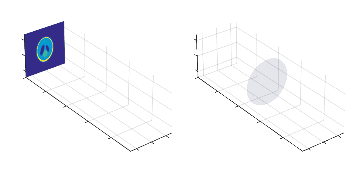
As the wavefield propagates it diffracts, and the image is rapidly distorted to the point where it is unrecognisable. It encounters a lens, 2 focal lengths away from where it started. The light is focussed down, before re-expanding to form an image another 2 focal lengths away. This is known as a 4f imaging system, for obvious reasons. In a laser laboratory (for example) it is used to ‘re-image’ a beam from one place to another. If left to its own devices, a laser will quickly diffract, which ruins the beam quality.

The image is a reversed version of the object, and in this special case has unit magnification. Between the lens and the image the light reaches a focus of finite size, whereas in the geometric optics limit the focus would be infinitely sharp. The focal plane can be shown to contain a spatial Fourier transform of the object, and messing with the light in this plane causes funky effects.

Isosurfaces

While it’s fun to examine how light propagates to form an image, it’s more fun to generate interesting shapes. Above I plotted alongside a set of isosurfaces of light intensity. These map surfaces of constant intensity over the calculated 3D distribution of light. Let’s have a look at another clearer version of the above:

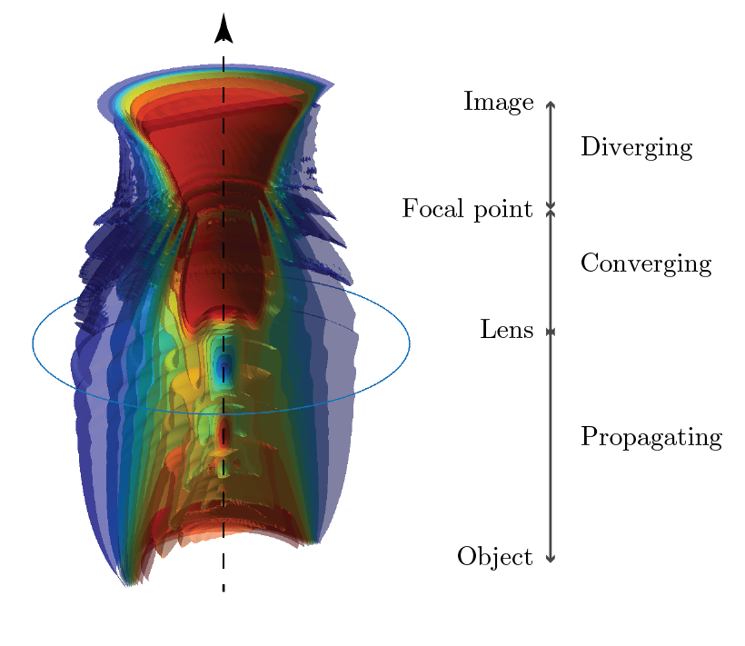
I’ve cut the surfaces in half to better detail their internal structure. I’ve also used a simpler object – just a plain circle. As the beam diffracts we see some interesting near-field structure – local maxima and minima along the optical axis, as the edges of the beam propagates away. As the beam hits the lens and focusses the diffraction is undone, and we see the outer ‘rings’ in the beam travelling back to the centre.

Rendering

I promised pretty images, but have hit the limit of what Matlab can provide. To go prettier we need some other tools. The first I tried was Drishti – a great tool for visualising 3D datasets, typically those from medical imaging. Using it on the Shepp-Logan dataset above, the view looks like this:

Now there’s much to be done with the colourmap here, but as a default result it’s quite striking how much detail can be resolved.

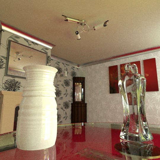
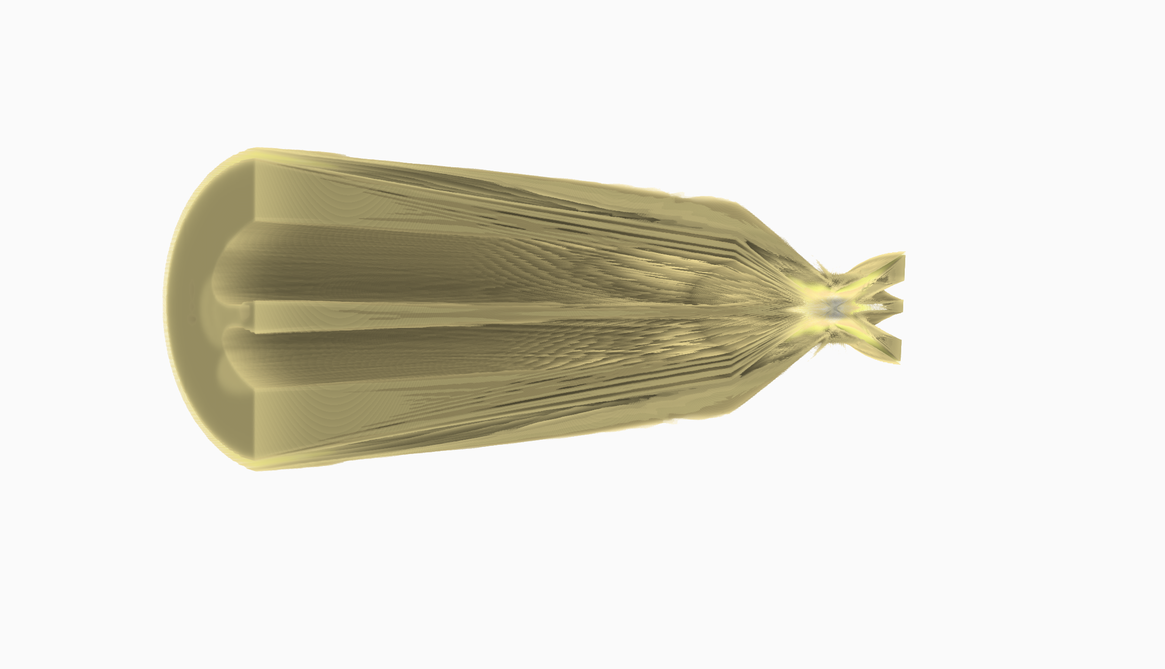
The other approach is to re-render the isosurfaces. Here I use Blender to import an .stl mesh of the isosurface and light the scene with a couple of lights:

Much better! Making the mesh a little transparent doesn’t hurt the overall look either.

Fourier Vases

Taking the full outer isosurface from above, I decided it looked a bit like a vase. It would be trivial for an owner of a 3D printer to print out one of these, and might make for an interesting conversation piece? Perhaps you could print the isosurface corresponding to an image of your own face? As for what it would look like sat on your dining room table, fortunately I had a .blend file lying around just for such a purpose: