Given a few of my previous posts it’s obvious that I’m a fan of the physics and mathematics that that comes along with the theory of classical optics. To make the number of lens-based posts a nice round three then, here’s a simple Matlab App I made over the last few days which lets you play with lenses interactively, hopefully giving a bit of useful insight into the underlying principles.

App Features

First of all then, you can get the app here, imaginatively called LensLab:

Mathworks File Exchange

You’ll need a copy of Matlab which supports ‘apps’, it was packaged with version R2014b and it should install into your App ribbon button area.

When you click the icon, you should be presented with the following:

The red lines represent collimated light rays (e.g., a laser), and the blue lines represent diverging light rays (i.e., those reflected from an object). We assume an object is placed at 0 on the x-axis, and the location of the image is represented by the dotted black line. The magnification of the image is written alongside (if the image is virtual, the magnification will turn red).

In the default configuration we have a simple imaging telescope, where two lenses are separated by the sum of their focal lengths and the outgoing laser beam remains collimated – this is impossible to do with a single lens.

We can move one of the lenses by clicking and dragging – when the lens bounding box turns blue a mouse drag will translate it on the x-axis.

We can also adjust the focal length of the lenses – by dragging near the edge of the bounding box the lens focal length is varied with mouse position. By moving the mouse behind the lens, the focal length can be negative, causing rays to diverge.

The buttons on the left allow the adding and deletion of lenses:

With a little playing around it’s easy to come up with relatively complicated designs:

To do

This is only a quick and simple utility (though I did spend longer than I’d like to admit playing with the figure properties…), so it doesn’t have many features. In the future, it is simple enough to add saving/loading, axis scaling, precise control of lens properties etc.

That being said, no one is going to use this for serious purposes, so enjoy mucking around with lenses for a bit. If there are any serious bugs, leave a comment either here or on the File Exchange submission. Some day, in the dim and distant future, I may even get around to getting everything on Github and you can fix the bugs yourselves, you lazy sods.

The ‘physics’

As said above, the ‘raytracing’ done here is really very simple. Each lens is assumed to be infinitely thin, which means its focal length is related to the radius of curvature of each side by

and I’ve also taken which makes things even simpler. I’ve also neglected the finite wavelength of light, so light is represented geometrically by ‘rays’ – straight paths it takes between optical elements. In this case, it is very simple to calculate the light paths using ‘transfer’ or ‘ABCD’ matrices (seriously, ABCD?).

If the ray is currently a distance from the optical axis and travelling at angle , its state can be represented by a vector

An optical element such as a lens changes the angle of a ray. Free-space propagation can be thought of another element which changes the distance but not the angle. The transfer matrices for these two elements are

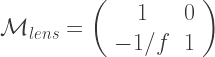
and the ray path is built by successively applying these transfer matrices, e.g.

and so on. On the plus side, this is very simple computationally and therefore fast. On the downside it is difficult to assess the performance of an optical system this way, unless many more factors are taken into account (see for example Zemax).

It might be fun one day to add support for aspheric/achromatic lenses, but the ‘fun’ factor isn’t much different, which means I probably won’t 🙂