It’s done! After 58,627 words, 233 pages, 369 references, 162 figures and 3 lonely tables I finished my PhD thesis. Weighing in at 161.8MB, it was unceremoniously uploaded and that was that. Here are a few tips and observations I made on the way, which are probably only useful to those of you battling through a long Latex document. Never fear, normal blogging service will resume shortly.

Content

The thesis title was ‘Diagnosis and Application of Laser Wakefield Accelerators’, and concerns a new type of particle accelerator technology based around high-power lasers. I won’t go into the details in this post, though data from a chapter of the thesis has been published in this open access paper for the terminally interested, which should probably be the subject of another post some time in the future.

While I’m not going to make the thesis text available until after we’ve published some of the unpublished data it contains, I did play around with a few summary visualisations.

Visualisations

Here are the word clouds corresponding to each chapter:

These were made with the fun wordcloud python module I’ve used before on this blog. The whitespace numbers were incorporated by generating an image mask to use with the module.

I also used the ImageMagick utility to convert the PDF of the thesis into a series of PNGs, before concatenating the images into an animated GIF:

Finally, given the existence of PNG images of each page, I did what any right-minded person would and analysed the colour content of the pages. I first transformed the colours to HSV (Hue, Saturation, Value) space, then for all the 116 million pixels in the PNG-ified thesis binned into 2D histograms over (H,S), (H,V) and (V,S):

The histograms are plotted on a log scale, as otherwise they are dominated by the main black and white colours of the images. On all three histograms there are obvious ‘traces’ through colour space, indicating the use of colours which join up neatly along a line. These are due to the colourmaps of the plots in the thesis, where 1D data is converted to a colour value by interpolating  it along a 1D line in 3D colour space. Two of my favourite colourmaps are indicated alongside, from the brewermap Matlab utility.

Writing the thesis

Dealing with a document this size involving lots of equations, references and vector graphics means the best solution is Latex. I used the TexStudio application, enjoying the nice default features of auto-completion, label tracking, citation lookup, viewing equations on hover etc. No doubt other people have their own favourite tex configuration with lots of customised shortcuts and utilities, but this worked pretty well for me out of the box. Here are a few changes I made to the default styles.

The main change was to make the section headings sans-serif throughout the thesis. I found the visual distinction against the serifed fonts of the main text helped the headings to stand out. Here I used the titlesec package, and the command I used to change the section style is

\usepackage[compact]{titlesec}

\titleformat{\section}[hang]{\fontfamily{phv}\selectfont\bfseries}{\thesection\hsp}{0pt}{}{}
\titleformat{\subsection}[hang]{\fontfamily{phv}\selectfont}{\thesubsection\hsp}{0pt}{}{}
\titleformat{\subsubsection}[hang]{\fontfamily{phv}\selectfont\itshape}{\hsp}{0pt}{}{}

You’ll notice I didn’t use the standard Latex sans-serif, but used Helvetica via the command

\fontfamily{phv}

Contents

Moving on to the contents page specifically, I used the tocloft package to tweak some styles. For a more compact listing I set the depth to be 1:

\setcounter{tocdepth}{1}

I changed the default separator from dots to a continuous line by cheating a bit:

\renewcommand{\cftdot}{\textcolor[gray]{0.75}{--}}
\renewcommand{\cftdotsep}{0}

The separator is a full-width hyphen, with no gap between the characters.

I made the chapter titles Helvetica

\renewcommand{\cftchapfont}{\fontfamily{phv}\selectfont\bfseries}

and stylised the page heading to include a frivolous vertical bar which matches the chapter headings

\renewcommand{\contentsname}{C \hsp \textcolor[gray]{0.75}{ \rule[-0.75ex]{0.08ex}{1.5em} }\hsp Contents}

Main chapters

The chapter headings were fiddled with using the titlesec package, where I inserted a vertical bar and shrank the whitespace beneath the title, which by default is massive.

\titleformat{\chapter}[hang]{\Huge\fontfamily{phv}\selectfont}{\thechapter\hsp{\textcolor{gray75}{\rule[-0.75ex]{0.08ex}{1.5em}}}\hsp}{0pt}{\huge\bfseries}{}

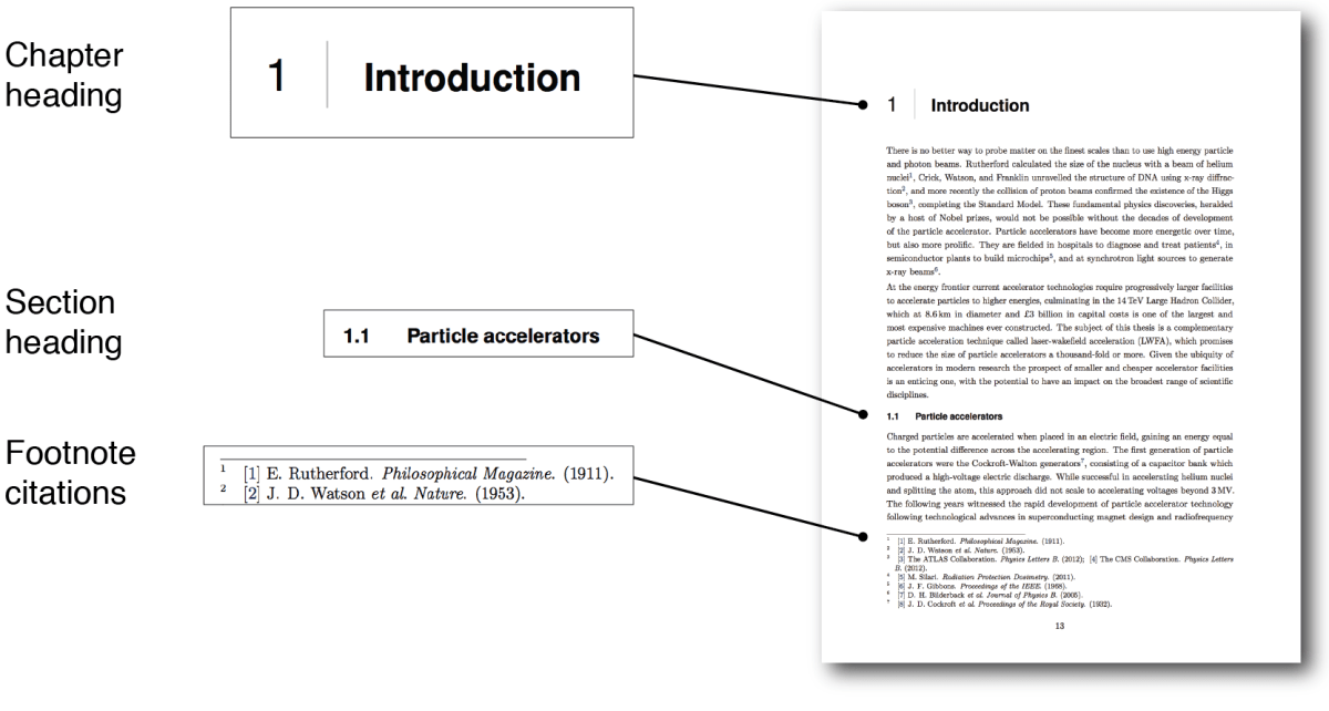
The footnote citations are enabled by the biblatex package. Here I overwrote the default cite command, using

\DeclareCiteCommand{\cite}[\mkbibfootnote]
{\usebibmacro{prenote}}{
	\usebibmacro{citeindex}
	\mkbibbrackets{\usebibmacro{cite}}
	\setunit{\addnbspace}
	\printnames{author}
	\setunit{\labelnamepunct}
	\printfield{journaltitle}
	\newunit
	\printfield{year}
}
{\addsemicolon\space}
{\usebibmacro{postnote}}

I wanted the footnote citations to be compact, so stripped out other details. The full citation was still contained in the bibliography. I made sure the year was bracketed using

\DeclareFieldFormat[article]{year}{(#1)}

I ensured that only the name of the first author was written using maxcitenames=1 in the biblatex options, and added the et al. using

\DefineBibliographyStrings{english}{andothers={\emph{et al}\adddot}}

Finally, to access the full citation the number was hyperlinked using the hyperref package, which if included allows biblatex to hyperlink citations by default. Borders around hyperlinked text were removed using

\hypersetup{colorlinks=true,pdfborder={0 0 0},citecolor=darkblue,linkcolor=darkblue,urlcolor=darkgreen}

where the default link colours were defined using the xcolor package

\usepackage[usenames,dvipsnames]{xcolor}
\definecolor{darkblue}{RGB}{0,0,90}
\definecolor{darkgreen}{RGB}{0,80,0}

Headers

Changes to the page headers are easiest with the fancyhdr package. In this thesis to avoid clutter I put the current chapter and current section on opposite pages, such that with the physical document open the current chapter and section are always visible. The following snippet does this, along with changing the font and removing a trailing dot after the section number (to match the section titles).

\usepackage{fancyhdr}
\pagestyle{fancy}
\renewcommand{\headrulewidth}{0pt}..
\renewcommand{\headrulewidth}{0.5pt}
\renewcommand{\footrulewidth}{0.0pt}
\renewcommand{\chaptermark}[1]{\markboth{\fontfamily{phv}\selectfont\chaptername\ \thechapter:\ #1}{}}
\fancyhead[LE]{\fontfamily{phv}\selectfont \leftmark}
\fancyhead[RE]{}
\fancyhead[LO]{}
\fancyhead[RO]{\fontfamily{phv}\selectfont \nouppercase\rightmark}
\renewcommand{\sectionmark}[1]{\markright{\arabic{chapter}.\arabic{section} \, #1}}

Figures

My figures were mostly made in Matlab, which has notoriously poor support for producing nicely-formatted vector plots. I persevered though, and found that using the print command to produce .eps files I could get decent results which remained editable in Adobe Illustrator. The standard Latex computer modern fonts are available in Matlab by setting the Interpreter property of a text object to Latex. On OSX the default Latex fonts can be found in

/usr/local/texlive/2015/texmf-dist/fonts/type1/public/amsfonts/cm/

I changed the figure caption title font to Helvetica, and ensured that the caption was ‘hanging’, i.e. did not extend beneath the title. This was done with the caption package

\usepackage[format=hang]{caption}
\renewcommand{\captionlabelfont}{\fontfamily{phv}\selectfont\bfseries\small}

Bibliography

Finally, given the number of references was quite large, I used an external reference manager called Mendeley. Mendeley has an option to produce a .bib file for your PDF collection, from which Biblatex will produce a .bbl file as appropriate for your document. I redefined some default bibliography drivers, as they are known in Biblatex, for formatting the bibliography entries.

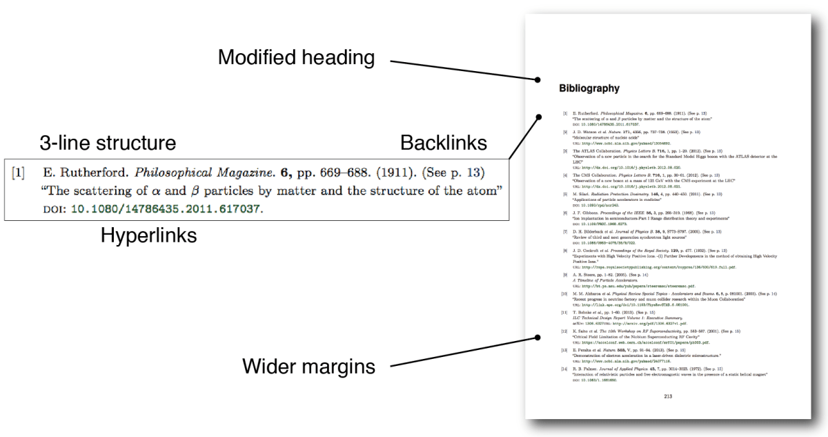
The bibliography heading inherits the chapter styling, so fit in with the rest of the document automatically. I did widen the margins, shrink the font size and remove the headers to minimise the bibliography page length, using the following commands before the bibliography

\newgeometry{top=1in, bottom=1in, left=1.0in, right=1.0in}
\renewcommand*{\bibfont}{\scriptsize}
\pagestyle{plain}

To change the style of the entries, I defined the bibliography driver as

\DeclareBibliographyDriver{article}{
\usebibmacro{bibindex}
\usebibmacro{begentry}
\newunit\newblock
\printnames{author}
\newunit\newblock
\usebibmacro{journal}
\newunit\newblock
\printfield{volume}
\newunit\newblock
\printfield{number}
\newunit\newblock
\usebibmacro{note+pages}
\newunit\newblock
\printfield{year}
\newunit\newblock
\usebibmacro{pageref}
\newline\newblock
\printfield{title}
{\iffieldundef{doi}{
    {\iffieldundef{url}
    {}
    {\newline\newblock
    \usebibmacro{doi+eprint+url}}
    {}
    }
}
{\newline\newblock
\usebibmacro{doi+eprint+url}}
{}
}
\finentry}

with different definitions for, e.g., books or conference proceedings. The backlinks are hyperlinks to where each entry has been referenced, using the backref=true option in Biblatex. The backlink text was altered using

\DefineBibliographyStrings{english}{
backrefpage = {see p.},
backrefpages = {see pp.}
}

For the external links, I preferentially printed URLs before DOIs by redefining the bibmacro

\renewbibmacro*{doi+eprint+url}{
\iftoggle{bbx:doi}
{\iffieldundef{url}{\printfield{doi}}{}}{}
\iftoggle{bbx:eprint}
{\iffieldundef{doi}{\usebibmacro{eprint}}{}}{}
\iftoggle{bbx:url}
{\usebibmacro{url+urldate}}{}
}

Hyperlinked figures

In the past when reading a thesis, I’ve occasionally wanted to replot a figure, or otherwise gather numerical data from it. This has usually meant using a service like WebPlotDigitiser, which lets you manually extract data by clicking on a rasterised image of the plot. This works, but is clunky and slow, can’t be automated easily, and, well, feels a bit grubby. I decided there would be no such awkwardness in my shining tome, and so added hyperlinks to my figures which took the reader to an online vector graphic or Matlab .fig file (which contains the data).

The figures are hosted on my Dropbox account, so I had to use the Dropbox python API to get public links to each figure. This is amazingly easy, e.g. to create a line in Latex which includes a hyperlinked figure one could use something like

import dropbox

token = 'private token'
dbx = dropbox.Dropbox(token)
share = dbx.sharing_create_shared_link(path='/path/to/file')
newline = '\href{share.url}{\includegraphics{/path/to/file}}'

where your private token comes from your Dropbox developer account page. I wrote some other functions to extract figure definitions from my Latex files, find the associated .fig file if it existed, and copy the relevant file to a Dropbox folder. The snippet above then wraps all \includegraphics lines with a \href, and that is that.

What now?

Excellent question. I’ve been fortunate enough to have been offered a position at Imperial College for the next year or so, and with any luck I’ll continue doing science after that.

I can be certain about one thing though – that I will forever be fascinated by the quirks of physics, mathematics, and patterns in data, and that when I come across something fun it will inevitably end up here.