img cmprssn w/ svd

Let’s get pedagogical. Often when analysing a system, it is useful to break a component down into pieces, and figure out which are the important ones (if any). There are many techniques for this, here I’ll look at one called ‘singular value decomposition’ in the context of image compression.

Let’s start with the usual dry explanation of singular value decomposition (SVD). For any $m\,\times\,n$ matrix $\mathsf{M}$ , it is possible to write $\mathsf{M}$ as

$\mathsf{M} = \mathsf{U} \cdot \mathsf{D} \cdot \mathsf{V^T}$

where $\mathsf{U}$ is an $m\,\times\,m$ matrix, $\mathsf{V}$ is an $n\,\times\,n$ matrix, and $\mathsf{D}$ is a diagonal matrix, i.e. a matrix that is non-zero only along the diagonal.

Writing this in index notation, we have

$M_{ij} = U_{ik}D_{k\ell}V^T_{\ell j}$

and letting the diagonal elements of $\mathsf{D}$ be $d_k$ ,

$M_{ij} = U_{ik}d_k\delta_{k\ell}V^T_{\ell j}$

or in another way and reintroducing the suppressed summation sign,

$M_{ij} = \Sigma_{\ell} d_{\ell} (\mathbf{u}_{\ell})(\mathbf{v}_{\ell})^T$

where $\mathbf{u}$ and $\mathbf{v}$ represent the column vectors of the matrices $\mathsf{U}$ and $\mathsf{V}$ . Intrigued? You shouldn’t be, because that’s not a very interesting way to look at the problem.

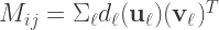
What is interesting is the way I’ve intentionally written the final step of the decomposition – to construct $\mathsf{M}$ , you just take a weighted sum over outer products of 1D vectors. The reason that this is interesting is that if you sort the weights – $d_{\ell}$ in this case – then by starting with the largest weights you gradually make a better and better approximation to $\mathsf{M}$ in the summation.

Let’s illustrate this with an example – image compression. Take the following grayscale image, famous in image processing circles:

This is a 2D array of numbers, or in other words, a matrix. We can therefore compute the SVD of this image, and reconstruct it from successively larger numbers of vectors $\mathbf{u}$ and $\mathbf{v}$ .

The following images and animation show how adding more vectors to this sum makes a gradually more faithful representation of the original matrix (image). In this case there are 512 $\mathbf{u}$ and $\mathbf{v}$ vectors, but even using 100 of them, the reconstruction is very close to the original image.

Hopefully you now understand both outer products and SVD a lot better. The top-left image in particular illustrates the outer product well: take some vectors along the left and top of the image, smear them across and down respectively, and multiply them together. This forms a 2D image from a pair of 1D vectors.

Features which are strongly horizontal or vertical are recreated the quickest, including the horizon and the tower in the background.

To understand how the accuracy improves as the reconstruction process proceeds, the next plot shows how the ‘amplitude’ ( $d_{\ell}$ ) falls with $latex \ell$.

I’ve marked a few points to discuss how the scaling varies. The orange point shows that the ‘low’ order (small $\ell$ ) vectors contribute most to the image, having large $d_{\ell}$ .

After the green point a large portion of the image is accounted for, and by the red point the weighting factors are so small there’s almost no point having them.

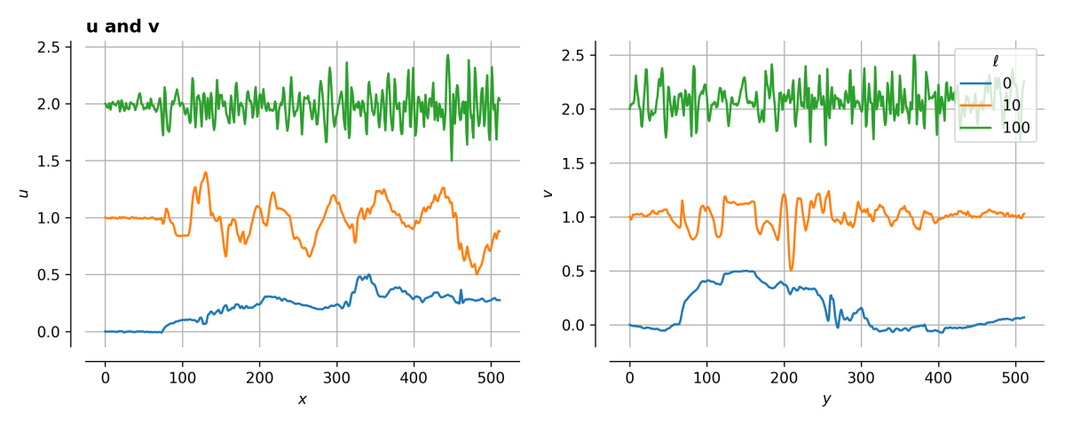
If we look at the vectors themselves, we can see below that low- $\ell$ vectors tend to vary slowly, and high- $\ell$ vectors vary much more quickly – i.e., contain information at high spatial frequencies.

This means that the general structure of the image is encoded in the low- $\ell$ vectors, and the high- $\ell$ vectors fill in the gaps. This is why one can think of SVD as a form of compression – throwing away imperceptible high-frequency information allows you to record fewer bytes, without degrading the visible detail in the image.

One way to characterise the performance of any compression method is to see how the error in the reconstructed image varies with the image size.

Here, the image size $S$ after SVD for an $N\,\times\,N$ image is

$S = \ell_{max}(2N + 1)$

where $\ell_{max}$ is the number of vectors to use to reconstruct the image. If this quantity is less than $N^2$ then the compression has been effective.

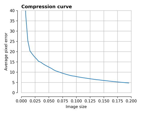
We see that for $\ell_{max} > 50$ , $S < 0.2N^2$ and the average error in pixel value is smaller than 5. This is nice! But can we do better?

One thing you might notice is that for this image, different areas will have different compression curves. Parts of the sky are very uniform, and so will be well approximated by a small number of vectors.

To test this, I also tried halving the image a number of times $p$ in the horizontal and vertical directions, and reconstructing each sub-image separately.

The overall size of the image then becomes

$S_p = \ell_{max}\left(\frac{2N}{2^p} + 1\right)2^{2p}$

i.e. the individual vectors have shrunk, but there are more of them in the overall image.

The following set of images show reconstructions for increasing $p$ (horizontal) and increasing $\ell_{max}$ (vertical).

You can probably tell that the top-right quadrant of the image is constructed well very quickly, compared to the detail in the legs of the tripod. The compression curves are plotted below.

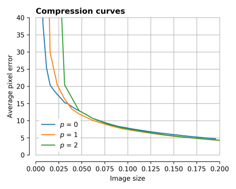
There is a very slight improvement – the orange and green curves dip slightly below the blue curve, but not much. We’re getting perhaps 10% improvement in either image size at a fixed pixel error, or pixel error at a fixed image size.

This is a bit disappointing, so let’s continue.

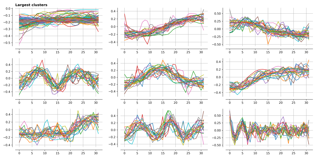
One thing that I noticed is that amongst the sub-images, several of the vectors computed for different SVDs looked quite similar. My idea was then to see if there were any ‘characteristic’ vectors which could be re-used across different sub-images, thereby saving the storage space of lots of similar vectors.

I used a method called k-means clustering here, but many algorithms exist, possibly with better performance.

Below I’ve plotted the 9 largest clusters, and it is clear that many vectors have similar forms – roughly uniform, increasing to the right, increasing to the left, single humps, double humps… to those of you who have done any Fourier analysis this should all look very familiar!

Finally, lets look at the performance of clustering compared to ‘simple’ SVD. The following plot is complicated, and shows several things:

The compression curve of simple SVD – plotted as open circles
For each $(\ell_{max}, p)$ pair, there is a line for the cluster model, along which the number of clusters increases. As the number of clusters reaches $\ell_{max}$ , these lines tend towards the simple SVD points.
Confusingly, in this plot I’ve called $\ell_{max}$ $n_{max}$ , and I’ve called $p$ $N_{levels}$

This time there are some significant performance improvements at the lower image quality settings – a 6-fold savings in image size in some cases – see the following comparisons.

Admittedly these images don’t look great compared to the original image, but they do demonstrate the conceptual point that it is possible to find repeated or irrelevant information and remove it – essentially the basis of all compression techniques.

I think this is quite nice, and there are a few further avenues for improvement. For example,

Different clustering algorithms
Different $\ell_{max}$ for different regions
Optimising the clustering
Picking sparse representations of vectors, or sparse representations of differences from clustered vectors
…

I’m sure this is all covered in various image compression formats somewhere (usually a generous commenter will tell me this kind of thing), and I know that JPEG in particular uses a discrete wavelet transform for example, but it’s always fun to try and have a go by oneself!

Almost looks like work

img cmprssn w/ svd

Leave a Reply Cancel reply

Share this:

Like this:

Related

Leave a Reply Cancel reply