This post is a classic example of the malady known as Jason-itis – idly wondering about a thing, and then having to dive deep down a rabbit hole to satisfy a geeky wish. In this case the thing was ‘I wonder how you make a 3D shape which looks like different shapes from different angles’, and the rabbit hole bottomed out at this GPU-accelerated demo. Let’s look at the stuff in-between.

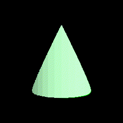
To illustrate what I mean, here’s an example of a 3D shape I made in Blender, the projection of which looks like a square, triangle, or circle depending on which angle you look at it:

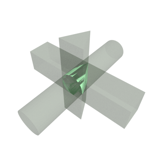
To construct this shape, I used a boolean operation: overlaying three volumes, and finding their intersection. This is the volume occupied by all three shapes simultaneously:

It would be fun, I thought, to be able to specify the desired cross-sections, and have something generate the required 3D shape (if it existed) in real-time.

Dealing with all of the details of creating a mesh with the right vertices etc. sounded painful though. Fortunately, I had been reading recently about a different kind of 3D rendering technique which makes these kind of boolean operations trivial – signed distance fields.

Signed distance fields (SDFs)

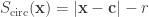
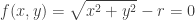
This is a fancy name for something very simple. An SDF is just a function which takes a position as an input, and outputs the distance from that position to the nearest part of a shape.

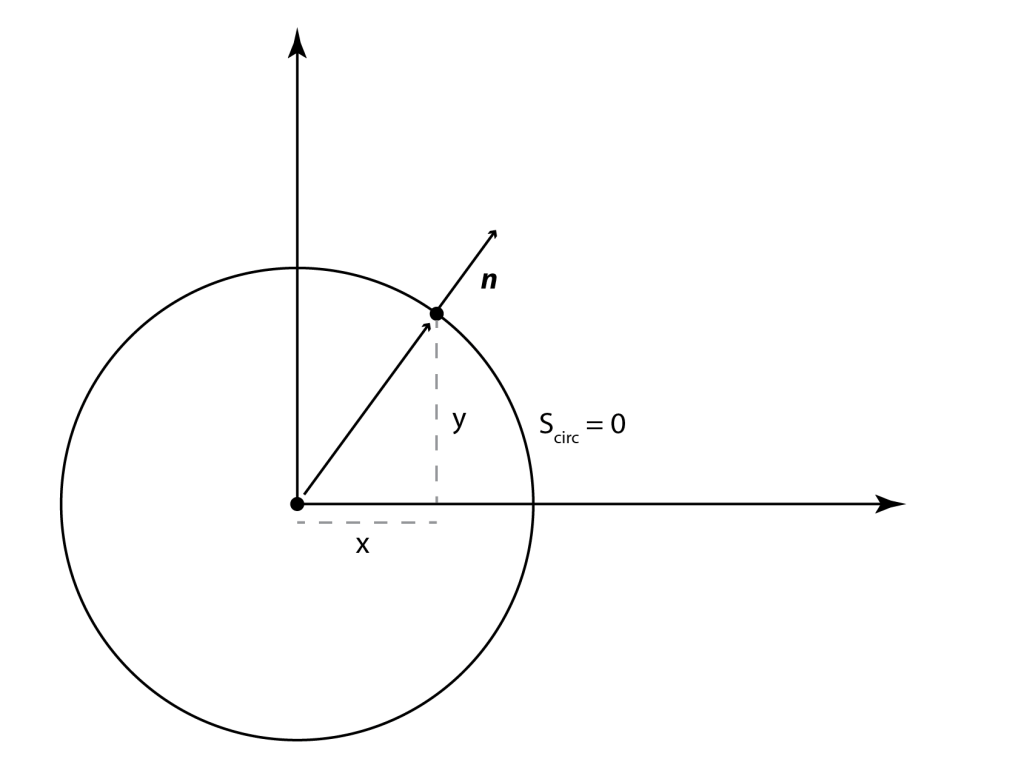
For example, the simplest possible SDF is that of a 2D circle, namely for a circle centred at with radius the function

gives you the distance to the edge of the circle. Let’s use this example to show how SDFs lend themselves to boolean operations.

Consider an object made of two, overlapping circles, with radii and centres subscripted with 1 and 2:

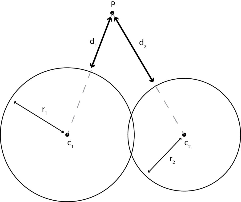
The question is, how are the individual SDFs combined to make a new, global SDF representing the joined object (the boolean union)?

Thinking about it for a second, we should first calculate the SDF for each circle individually – and . We should then return whichever circle edge is the closest, i.e.

This is cool, and there is a great list of SDFs for different primitive shapes listed here, but how do we actually draw the result of an SDF?

Rendering SDFs

The above examples were 2D, but we’ll be rendering 3D SDFs (i.e., a function of 3 coordinates). The diagram below shows how we’ll be thinking about the SDF during rendering.

The 2D viewport (transparent square) is between us (the ‘camera’) and the surface of interest represented by the SDF.

For each pixel in the screen, imagine sending a ray on a straight line from the camera to the pixel. Our task, as a renderer, is to figure out for each ray

• Does the ray hit the surface?
• If so, where, and at what angle is the surface?

If the ray doesn’t hit the surface, we just colour in the pixel white (or transparent). If it does, we need to know what angle the surface is at to know how to shade it. Let’s tackle these parts separately.

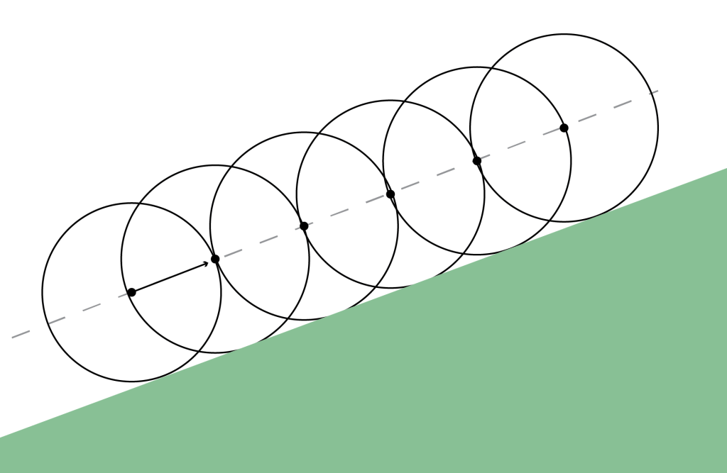
Does the ray hit the surface?

For each ray, we know where it starts and what direction it’s going in. If we ever know where it is, we also know how far it is to the surface using the SDF. Crucially, we don’t know in what direction the closest point of the surface is, so we have to figure that out by gradually stepping along the direction of the ray.

In the diagram below, we begin at the left heading along the ray indicated by the dotted line. The SDF is represented by the green circle.

We calculate the SDF, which means it must be safe to go at least that distance along the ray. We therefore travel that far, before stopping and re-evaluating the SDF. This process is called ray-marching.

In this case, we’ll actually never hit the circle and so the marching is truncated after a certain number of steps, or after a certain distance has been travelled. In other cases, we do hit the surface and so have to calculate the surface angle.

Calculating the angle of the surface

There’s a neat bit of maths it’s worth elucidating here, so I’ll go into a little detail. Consider some function which defines a surface .

If you move along the surface a small distance , then by definition the value of the function doesn’t change, i.e.

Because is small, we can expand the LHS in a Taylor series

Now is generic, so represents a small linear portion of the surface around . The above therefore states that is normal to the surface. Let’s convince ourselves with a simple example. Consider the ‘surface’ below of a circle:

The equation describing the circle of radius is

At the point , it is obvious that the normal to the surface is parallel to the position vector, i.e. .

Calculating the derivatives, we have

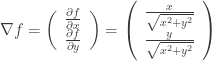
which is what we required above. This definition extends to more general functions, and so we can use it for rendering SDFs.

Considerations for the renderer

Let’s recap the steps we’ve gone through:

• It would be nice to easily calculate and render the boolean intersection of arbitrary volumes
• SDFs can be used to calculate intersections easily
• If you can write down an SDF, there is a way to draw it

The final, missing question to be answered is then

• How do you write down the SDF of an arbitrary volume?

I imagine there are many ways to solve this. The more mathematically inclined reader might start thinking about Fourier series, spherical harmonics, Sturm-Liouville theory, … (If you do have a good answer to this, let me know!)

My particular aim was to intersect extrusions, i.e. linear projections of 2D shapes. This simplifies the problem enough that I could have a go at solving it, but I’m sure there are better or more efficient solutions, and I’d like to hear about them!

On a computer, any 2D shape can be approximated by 2D squares, i.e. pixels. The obvious solution is then to rasterise the projection, and build up a complicated SDF from the union of loads of 3D boxes (for which there are known SDFs).

The only problem with this idea is that it takes many pixels to make a decent shape, and therefore the SDF gets very complicated and slow to render. The final final step before writing a my renderer then, is to be able to convert a 2D shape to a smallish number of rectangles.

Simplifying the SDF

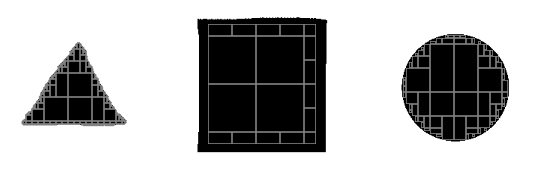
Let’s start with the answer – here’s an animation of a quick tool I wrote to fill in arbitrary pixelated shapes with rectangles:

For those interested, I’m using an HTML canvas, and simply manipulating the ImageData property to access the pixels as a raw array.

The process is simple – start with a big rectangle and keep splitting it up into smaller ones as required. In pseudocode, missing some details, it goes like:

rectanglesToProcess = [ (1 big rectangle the size of the canvas) ]
rectanglesToReturn = []

while there are rectanglesToProcess
  rect = rectangles.pop()
  is rect all black?
    rectanglesToReturn.push(rect)
  else
    quadrants = makeQuadrants(rect)
    rectanglesToProcess.push(quadrants)

return rectanglesToReturn

There are much better ways of doing this, but this approach was quick enough and made few enough rectangles that I could live with it.

Writing the renderer

The 3D renderer is written in webGL, which is a necessity if you want to do 3D visuals on the web with any kind of performance. Performance is pretty important here – for a 512×512 pixel image, rendering an object formed of around 500 boxes means evaluating an SDF about half a billion times. Doing this at 60 fps in serial would mean you have around 100 picoseconds per evaluation. Given that light only goes a centimetre or two in this time, parallelisation is the order of the day.

The rendering process in webGL happens in two steps

1. Vertices of geometric objects (triangles) are projected into 2D space – this is called the vertex shader
2. The pixels within the boundary of the projected geometry are coloured in – this is called the fragment shader

Both of these happen in parallel, and so each pixel must be able to be processed independently.

Step 1 is very simple here – we are only interested in the pixels, so the geometry just consists of a single rectangle filling the screen. Step 2 is more interesting – schematically it looks like the following

// pixel goes from -1 -> +1 across the viewport
vec2 pixel = 2. * (gl_FragCoord.xy / resolution.xy - 0.5);

// Initial position of the camera - l units away
vec3 initialPos = vec3(0.0, 0.0, l);
float angleX = pixel.x * fovX; // fov = field-of-view of camera
float angleY = pixel.y * fovY; // The 'angle' of each pixel
// Direction of camera ray
vec3 dir = normalize(vec3(tan(angleX), tan(angleY), -1.0));

// March the ray to the surface
vec3 marchResult = rayMarch(initialPos, dir);

// Get the normal the surface
vec3 n = normal(marched, dist);

// ... colour in the pixel

There is a slight technical quirk, to do with passing the information about the rectangles to the GPU. In webGL there is the concept of ‘uniforms’ – data that every pixel can access. Unfortunately there is an upper limit on the size of the uniforms which can be passed to the fragment shader, which in my case was often smaller than required to accurately render an object.

To get around this, the information about each rectangle was packed into an image texture. The 4 numbers describing a rectangle (x, y, width, height) can be associated with the (red, green, blue, alpha) properties of a pixel. This texture can then be sampled inside the fragment shader, which gives us a much larger size limit, but is a slower operation.

The results

Right, enough dry technical stuff – let’s look at some pictures. You can also have a play at https://jasmcole.github.io/Pages/CSG with a decent GPU. Your phone might struggle though!

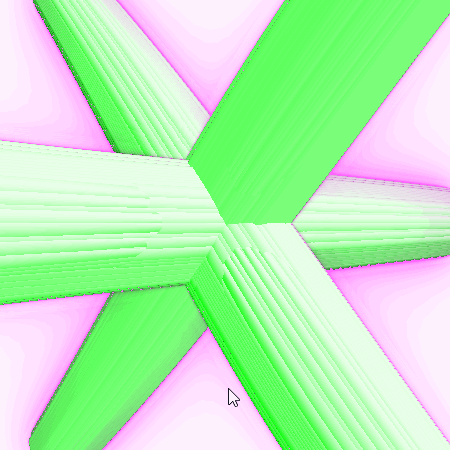
Here is the default view, corresponding to the extrusion of 3 circles:

The surface representing SDF = 0 is coloured a tasteful green. The intensity of the magenta surrounding the edges correponds to the number of ray-marching steps required for each pixel – up to 50 are attempted. The reason that the number of steps goes up near the edges is due to the fact that marching parallel to the surface is extra expensive, as the maximum allowed step size is small:

This is especially apparent when extrusions are nearly face-on:

The view can be rotated/zoomed, and intersections turned on and off:

With default settings, on a good GPU it’s possible to edit the SDF interactively, which is pretty fun:

OK, let’s see if we can get close to the Blender example at the beginning. Below I’ve attempted to draw a triangle, square, and circle. The generated rectangles look like this:

and the intersection made from the SDFs is reassuringly familiar:

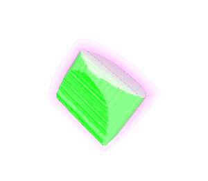
Which is to say, I spent a long time replicating something to a lower standard than I started with.

Good fun though.

Code

You can get the code to the web app here:

https://github.com/jasmcole/Blog/tree/master/CSG

It is a minimal React / Typescript project. The webGL is written from scratch, so it could serve as a useful minimal fragment-shader-only base example.

Resources

There were a few excellent blogs and websites I used to get me going with this:

• http://www.iquilezles.org/index.html – an excellent repository of information on SDFs and other 3D techniques
• https://www.alanzucconi.com/2016/07/01/signed-distance-functions/#part4 – good animations
• http://jamie-wong.com/2016/07/15/ray-marching-signed-distance-functions/ – the blog post I originally read which got me thinking about SDFs
• https://github.com/paulirish/webgl-boilerplate/blob/master/index.html – this very helpfully reminded me of the webGL boilerplate required to get going