Here’s a post which combines my favourite bits of writing a blog – fairly mathematical, not too simple or difficult to implement, mostly based around pictures, not covered in my undergraduate education, and pretty damn useful in my job. Excited? You should be.

Inverse problems

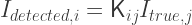
It’s important to be regular, in many aspects of life, but most importantly of all when dealing with ill posed problems. I’ll come onto a specific example later, but for now consider the general matrix problem

where the information contained in is known, and we would like to recover . The matrix is determined by the physical system under analysis, where the physical quantity is mapped under some linear transformation to a quantity which is measured.

This is a matrix equation, so the answer is simple right? Just find the inverse of and apply it to both sides

Formally, this answer is correct and recovers exactly. However this is the real world and so we don’t know exactly, it is associated with some error . To see how the solution we recover varies as is altered, denote the error in as then

for some norm . Given that then the fractional error is bounded by

The scaling between the errors in the inputs and outputs is known as the condition number of the matrix

If is large, then even tiny errors in the measurement can generate large errors in the output. A matrix with large condition number is said to be ill-conditioned and such a problem ill-posed.

This is generically known as an ‘inverse problem’, where the ‘forward transform’ is known but the inverse transform problematic or impractical to calculate directly. Many problems can be translated into an inverse problem, a notable example being computed tomography which occupied a portion of my PhD.

Image deconvolution

Here let’s look at the simpler example of image deconvolution. When taking a picture, the ‘true image’ will be smeared across the image detector due to imperfections in the detector. This smearing can be modelled by a convolution

for some point-spread function (PSF) (also known as a kernel). The PSF acts to mix up the image such that a given measured pixel contains contributions from many ‘true’ pixels, and the resolution is worsened.

To cast this as an inverse problem, write the images and PSF in terms of pixels

The PSF now takes the form of a matrix which relates how pixels of the true image contribute to pixels of the detected image. To recover the true image, one just needs to know the form of the PSF.

Lets do this. Below I construct a Gaussian PSF, generate its matrix, and apply it to an image to make a blurred image. I then invert the matrix, and apply that to the blurred image to recover the initial ‘true’ image.

Worked perfectly! What’s the problem then? Let’s add a tiny amount of noise to the blurred image, just 1 count on average (out of an 8-bit gray value range 0-255)

The blurred image looks, by eye, to be identical to the previous figure. The recovered image is utterly corrupted though, to the point where no semblance of image structure is maintained. What happened?

If I calculate the condition number of the matrix , I get . This is a very large condition number, and says that a 1% fractional change in the input image will generate a 100,000,000% change in the output image. This is, putting it mildly, unfortunate. To check I understand what’s going on, I computed recovered images for different levels of added noise and checked how far they were from the true image:

The blue line marks what should be expected given the condition number of ,  and clearly the recovered images follow this trend. To recover a recognisable image with error < 100, one requires an RMS measurement error of below 1 part in a million. This is very rarely achievable in practice, and demonstrates that this de-blurring technique will generally not work.

What is needed is a bit of regularisation.

Regularisation

The problem we are running into here is that, with some noise added, there can be many possible solutions for the recovered image. The large condition number of the matrix means that while 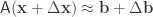,  it is not necessarily true that .

One solution is to penalise large values of to try and stop the recovered image shooting to infinity. The procedure is to then search for an which minimises

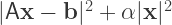
i.e. is close to a solution in a least-squares sense, but which also isn’t too large. The parameter determines the relative weighting of each term, and is known as a regularising parameter. This regularisation scheme is known as Tikhonov regularisation.

Differentiating the above with respect to the components of , we have

If then as expected. With non-zero though, it isn’t true any further that . If this condition is applied to the above, then

This relation can be interpreted as an iterative update, i.e. is updated iteratively as

In this case the iterates (hopefully) converge to a solution which better matches the measurement .

Regularised image deconvolution

Let’s finally see how well this technique works to de-blur images. Here Gaussian noise is added of magnitude 1:

If the noise magnitude is lower, the deconvolution is more successful:

If the noise magnitude is larger, the deconvolution isn’t very successful in improving the resolution, but it does lower the noise level:

In practise, the parameter needs a bit of fine-tuning for best results. It is also possible to generalise this approach, penalising other aspects of the image.

If, rather than the square of the image, the total variation  is penalised, the regularisation process encourages image uniformity (or ‘gradient sparsity’). This a technique widely used in computerised tomography, where it increases the quality of the 3D reconstruction without increasing the radiation dose to the patient.

Implementation

The code used in this post was written in Matlab, which deals well with large matrices. In particular the kernel matrix is large and sparse – for a 128×128 pixel image it is 16384×16384 and 99.5% sparse.

The scripts can be found here on Github. Keep the images small, even 128×128 takes a few tens of seconds to run.